Abstract:To minimize the inventory costs of detecting demand change, an acceptance/rejection method(threshold) is proposed. The proposed threshold can be identified by the newsvendor based on the excess cost, the shortage cost, the transitional probability of the demand change, and the magnitude of the demand change. Compared with the single exponential smoothing method, it is proved that the proposed method can save many more inventory costs when detecting a step change in demand. By analyzing the proposed method, it shows that as the magnitude of step change increases, the supply chain members turn to synchronously judge a step change, and as excess (shortage) cost increases, a newsvendor tends to respond slowly (early) to an increase in demand and responds early (slowly) to a decrease in demand. Observations from this study suggest that supply chain members should pay careful attention to different profit-margin products and different magnitude demand changes in cooperating and sharing demand information with others.
Key words:demand detection; demand change; inventory cost minimization; newsvendor
The ability to predict step changes in demand can never be overestimated. Often it may mean a difference between life and death for an enterprise[1]. Anecdotal evidence suggests that failure in detecting the underlying demand change may have disastrous consequences[2-3]. For instance, failing to predict strong market demand for the electronic book readers, Barnes & Noble Inc. suffered lengthy shortage and customers’ rage[2]. Nike lost $400 million with massive surplus shoes due to its slow response to demand decline[3].
In today’s business environment, step changes in demand can be triggered by factors such as promotions (e.g., price discounts, bundling with complementary product) and competitive events (e.g., competitors’ stockouts)[4]. In these situations, managers believe that a step change of demand is likely to occur but do not know when. To set inventory targets under demand uncertainty, the decision maker tends to use demand realizations in earlier periods to judge if a step change in demand has occurred. In reality, however, this demand data is often limited in terms of volume and/or quality and thus not sufficient for an accurate prediction of demand change[5].
Although software based on demand realizations has been developed to assist forecasting practitioners, they often complain about its inaccuracy. This is evidenced by a survey of 240 US firms, which shows only 11% companies use forecasting software and among them about 60% of the users modified the forecasts based on their intuitions[6-7]. This is specially the case when the manager anticipates a demand change and believes that the forecasts based on demand realizations are not as reliable as expected, and thus tends to rely more on other information to predict the demand change. For example, managers can use the text of financial news-headlines to predict the changes in the exchange market[8] or utilize online consumer reviews to predict the demand change of a hotel[9]. This kind of information can be used to predict the probability of demand change (called the transitional probability hereafter) thanks to the technology of big data analysis[8].
There are two approaches for the integration of the transitional probability and demand realizations[10]: voluntary integration and mechanical integration. In voluntary integration, the managers are provided with the statistical forecasts generated by demand realizations and decide how to use the statistical forecasts in judging demand change. In mechanical integration, the transitional probability is integrated with statistical methods to assist judgments of demand change. Syntetos et al.[11] went a step further by pointing out that the judgmental methods of demand changes should be evaluated with respect to the performance of inventory systems, and the integration approaches utilized in practice do not relate directly to their consequences on inventory costs. Therefore, it is paramount to analyze how to integrate recent demand realizations and transitional probability effectively to better predict step change with the aim of minimizing inventory costs.
In this paper, we intend to address the above research gap by considering a simple problem, where an inventory manager anticipates only one demand change. Assume the current period is period t. Two types of demand information (i.e. demand realizations x1, x2, …, xn and the transitional probability p) are available for judging step change. When ordering inventory under such demand uncertainty, managers face the risk of mismatching the supply and demand. How to avoid mismanagement so as to control the inventory costs effectively? A rational approach is to integrate the recent demand and the estimate from other sources when predicting demand change.
1.1 Step change model
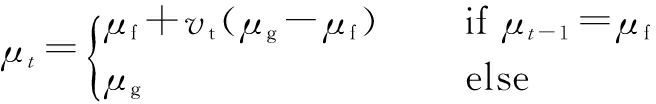
Let period t represent the current period in which the forecaster needs to judge the demand level and place orders. The period before period t is denoted as period t-1. Demand in period t is dt. Consider a newsvendor for a single product facing demand uncertainty. dt-1 and dt may be different. They can be represented by N(μf,σ2) and N(μg, σ2), respectively. The transitional probability is denoted as p. Correspondingly, the probability of no distribution change is 1-p. The demand process can be formulated as follows:
dt=μt+εt
(1)
(2)
where μf and μg are two constants representing the demand level before and after the step change, respectively; μt denotes the demand level in period t; εt is a random variable which follows a normal distribution N(0,σ2); vt is a random variable which follows a binomial distribution B(1,p).
There are three possible scenarios of the demand distributions in period t-1 and period t: (G,G), (F,G) and (F,F). Tab.1 shows the probabilities associated with the three demand change scenarios from t-1 to t.
Tab.1 Scenarios of the actual demand distribution
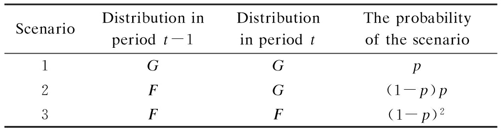
ScenarioDistributioninperiodt-1DistributioninperiodtTheprobabilityofthescenario1GGp2FG(1-p)p3FF(1-p)2
Not knowing the actual distribution, managers face the risk of assuming the wrong view on demand, resulting in poor replacement decisions and high inventory costs. To control costs, managers should make good use of the available information. In addition to p, management in fact also possesses the knowledge of the prior demand (xt-1, the realization of dt-1). To optimize inventory decisions, we propose a method to detect the demand change from the prior demand xt-1 and p.
1.2 Detection rules with prior demand
View the prior demand xt-1 as an indicative signal of demand level shift. The method that we utilize is the signal detection theory (SDT) approach[12-13]. The explicit objective of the newsvendor is to determine the existence or nonexistence of step change so as to minimize the expected inventory costs. According to the SDT, the following two heuristic rules are defined to detect the increase and the decrease of demand, respectively.
 .
.
Rule 2 When 0<μg<μf, if ![]() , then believe that the demand level in period t is μf; otherwise, believe that the demand level in period t is μg.
, then believe that the demand level in period t is μf; otherwise, believe that the demand level in period t is μg.![]() is the acceptance/rejection criteria. Parameter k is a real number, namely, the detection threshold.
is the acceptance/rejection criteria. Parameter k is a real number, namely, the detection threshold.
In this section, we first calculate the expected inventory costs under step change, and then derive the optimal detection thresholds, which can minimize the expected inventory costs.
2.1 Newsvendor model under step change
In a newsvendor problem, a newsvendor purchases units from a wholesaler at the same cost to resell at a given retail price in each sale period. The demand is random and unknown when orders are placed. If the order quantity is larger than the realized demand, the newsvendor has to pay the price for disposing of the remaining items. If the order quantity is smaller than the realized demand, the newsvendor foregoes some profit. Thus, the inventory costs arise in two ways as follows. When demand is less than the inventory ordered, the leftovers are often salvaged at a lower price and excess costs (ce per unit) should be paid. Alternatively, inventory shortage entails back orders and lost sales and the shortage costs should be paid (cs per unit). It can be clearly seen that, when management chases the prior demand xt-1 by adopting Rule 1 or Rule 2, the expected costs of different scenarios in Tab.1 vary. There will be six different forms of the expected inventory costs as shown in Tab.2.
Tab.2 The expected inventory costs
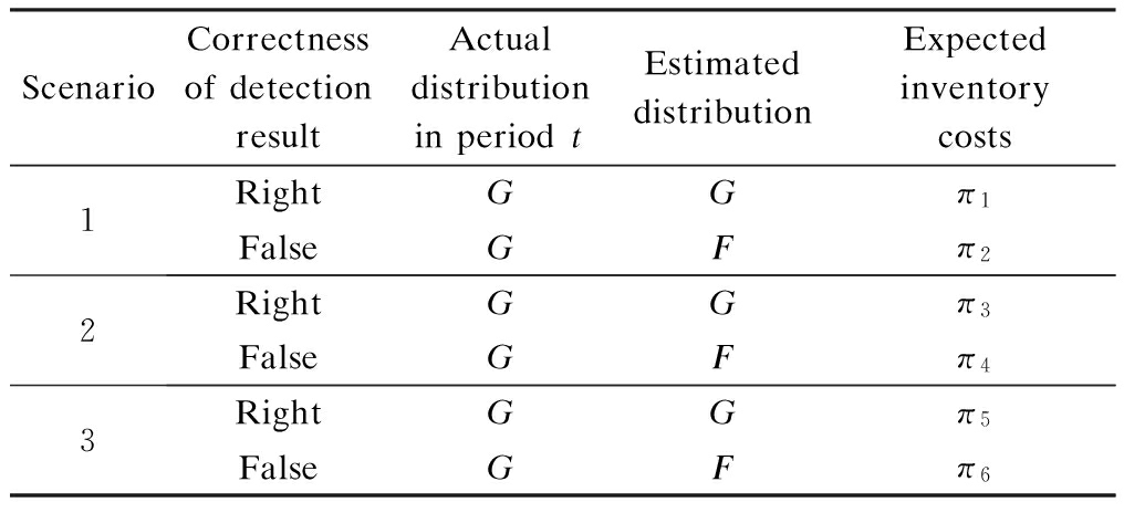
ScenarioCorrectnessofdetectionresultActualdistributioninperiodtEstimateddistributionExpectedinventorycosts1RightGGπ1FalseGFπ22RightGGπ3FalseGFπ43RightGGπ5FalseGFπ6
The order quantity is assumed to be the critical fractile solution and it can be expressed as ![]() , where
, where ![]() (·) denotes the inverse cumulative distribution function of random demand X. In Tab.2, πi(i=1,2,…,6) represent the expected inventory costs under both the actual and the estimated distributions given in each row. Due to the same combination in columns 3 and 4, we have π1=π3, π2=π4. It is worth noting that πi(i=1,2,…,6)are only determined by F, G and the cost parameters of the inventory system, and they can be calculated easily (The technical details can be found in Ref.[14]).
(·) denotes the inverse cumulative distribution function of random demand X. In Tab.2, πi(i=1,2,…,6) represent the expected inventory costs under both the actual and the estimated distributions given in each row. Due to the same combination in columns 3 and 4, we have π1=π3, π2=π4. It is worth noting that πi(i=1,2,…,6)are only determined by F, G and the cost parameters of the inventory system, and they can be calculated easily (The technical details can be found in Ref.[14]).
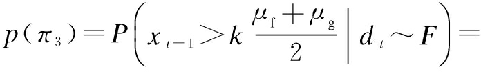
We next provide the probabilities of different expected inventory costs, which appear on the rightmost column of Tab.2, as shown in Tab.3.
Tab.3 Probabilities of expected inventory costs

ScenarioCorrectnessofdetectionresultActualdistributioninperiodt-1EstimateddistributionProbability1RightGGp(π1)FalseGFp(π2)2RightGGp(π3)FalseGFp(π4)3RightGGp(π5)FalseGFp(π6)
Due to the same actual demand distribution in t-1 and forecast, we have p(π3)=p(π6), p(π4)=p(π5). Furthermore, p(πi)(i=1,2,…,6)can be determined as

1-Φ
(3)
p(π2)=1-p(π1)=Φ
1-Φ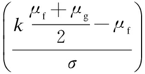
(4)
p(π4)=p(π5)=1-p(π3)=Φ
p(π6)=p(π3)=1-Φ
where Φ(·) is the distribution function of a standard normal distribution, and ![]() B) stands for the probability of event A given B. The total expected inventory costs under Rule 1 or Rule 2 can be expressed as
B) stands for the probability of event A given B. The total expected inventory costs under Rule 1 or Rule 2 can be expressed as
TC(k)=![]()
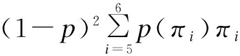
(5)
An optimal k can properly (economically) help to classify the prior demand xt-1into F or G, which in turn helps to make the right ordering decision and minimize the expected inventory costs.
2.2 The optimal detection of step change for newsvendors
![]() .
.
Theorem 1 The optimal detection threshold that minimizes the total expected inventory costs TC(k) can be determined as follows:
When μf<μg, the optimal threshold of Rule 1 is
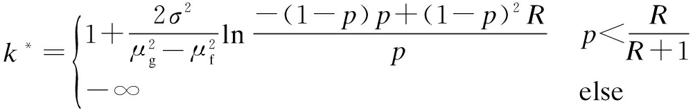
(6)
When μf>μg, the optimal threshold of Rule 2 is

(7)
![]() s.
s.
The optimal detection threshold k* depends on parameters p, μf, μg, σ, ce, cs. Due to the demand environments and cost parameters being dynamic (always changing) in practice, it is beneficial to make clear the relationship between k* and the transitional probability p, the magnitude of step change ![]() , the shortage cost cs, and the excess cost ce to the decision makers.
, the shortage cost cs, and the excess cost ce to the decision makers.
3.1 Optimal detection strategy vs. single exponential smoothing method
In practice, most firms use exponential smoothing models for forecasting demand that shifts over time[15-16]. Now, under the assumption of μf<μg, we show the advantage of the proposed detection rule by comparing it with a classic demand forecasting method—the single exponential smoothing method.
Before processing, we briefly introduce the process of the single exponential smoothing method. By using the single exponential smoothing method, forecast Ft+1 is a weighted average of the prior demand realization and the previous forecast.
Ft+1=Ft+α(xt-Ft)
(8)
where parameter α represents the weight of the forecast error xt-F. The optimal value of α can be determined as[15]

(9)
where W=var(xt)/σ2. According to the central limit theorem, through massive trials, it is logical to replace B(1,p) with N(p,p(1-p)). Thus, the corresponding value of W can be determined as

(10)
In this numerical example, the related parameters are set as follows: ce=100, cs=120, μf=4, μg=5, σ=1. Seven possible previous forecast values and ten levels of probability weight are considered. Specifically, Ft-1∈{3.0,3.5,4.0,4.5,5.0,5.5,6.0} and p∈{![]() n=0,1,2,…,9}. For every combination of Ft-1and p, we do 1 000 trials and record all the inventory costs in each trial. By the average expected inventory costs of different combinations, we compare the performance of the proposed optimal detection strategy with the single exponential smoothing method.
n=0,1,2,…,9}. For every combination of Ft-1and p, we do 1 000 trials and record all the inventory costs in each trial. By the average expected inventory costs of different combinations, we compare the performance of the proposed optimal detection strategy with the single exponential smoothing method.
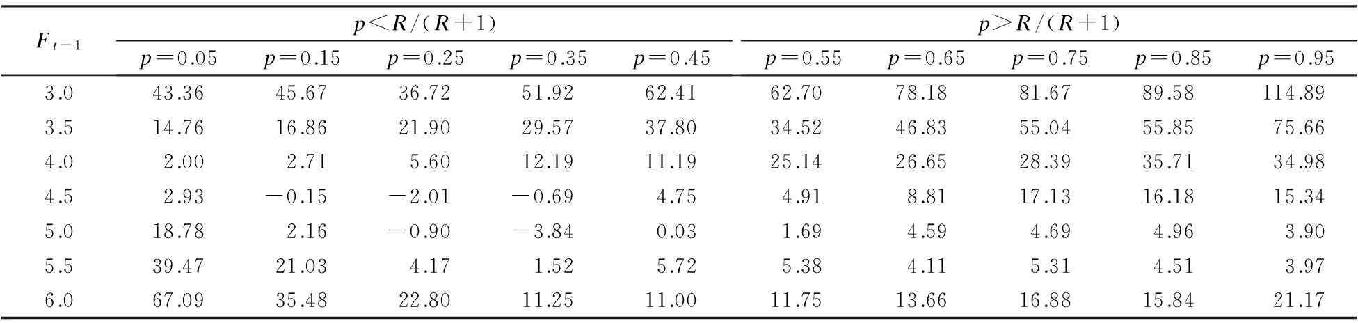
For each combination, the costs reduction of using the optimal Rule 1 to replace the exponential smoothing method is recorded in Tab.4.
Tab.4 Expected costs reduction by replacing exponential smoothing method with detection rule
Ft-1p
Tab.4 reports that the proposed detection strategy outperforms the exponential smoothing method for most of the combinations of Ft-1and p. The single exponential smoothing method operates with lower inventory costs only when the previous forecast is near to 4.5 or 5.0, and p is in a subset of the interval (0,R/(R+1)).
Forecast is a basic input in the decision process of operations management since it provides information on future demand. The importance of forecasting to operations management cannot be overstated. The primary goal of operations management is to match supply to demand. However, without completely knowing whether a step change occurs, matching supply to demand is difficult and may incur severe loss to businesses. Tab.4 shows that once a step change occurs, the averaging techniques are not a good choice. The proposed detection method can outperform the best averaging technique, the single exponential smoothing method, when the transitional probability satisfies certain conditions, in the sense of saving inventory costs. Thus, when facing a possible step change, it can be expected to reduce the inventory costs by applying the proposed detection method.
3.2 The impact of the magnitude of step change
Now, we numerically investigate the impacts of step change magnitude ![]() and transitional probability p on the optimal threshold k*. Specifically, study four different cases:
and transitional probability p on the optimal threshold k*. Specifically, study four different cases:
1) ce=9, cs=81, μf=100, σ=20, μg∈{110,120,130};
2) ce=9, cs=81, μf=100, σ=20, μg∈{70,80,90};
3) ce=9, cs=1, μf=100, σ=20, μg∈{110,120,130};
4) ce=9, cs=1, μf=100, σ=20, μg∈{70,80,90}.
Fig.1 displays the impacts of step change magnitude ![]() and transitional probability p on the optimal threshold k*, which shows that k* decreases with p when
and transitional probability p on the optimal threshold k*, which shows that k* decreases with p when
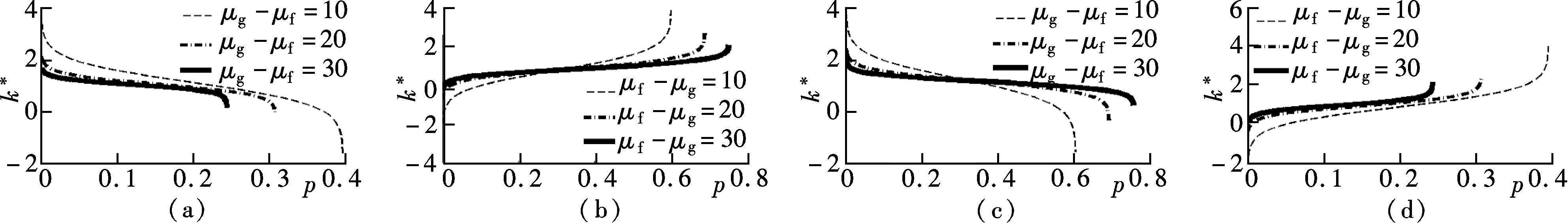
Fig.1 Impact of the magnitude of step change on the optimal detection threshold. (a) ce<cs, μf<μg; (b) ce<cs, μf>μg; (c) ce>cs, μf<μg; (d) ce>cs, μf>μg
ce<cs and increases when ce>cs.
In a retail supply chain people, step changes often result from promotions, which many people consider an essential part of doing business and the most prevalent means to stimulate consumer demand. In practice, both retailers and manufacturers execute a variety of retail promotions, such as, price discounts, in-store displays, and other advertising features[4]. To maximize the profit of the whole channel, supply chain members need to cooperate to forecast the demand influenced by promotions. Thus, the response of the other supply chain members is crucial for both manufacturers and retailers. Fig.2 shows that when facing an step change in demand, the optimal acceptance-rejection threshold k* limits to 1 as the step change magnitude approaches infinity. That is, even when supply chain members have different cost structures, they respond synchronously only if the magnitude of step change is large enough. Thus, when the magnitude of the step change is very large, the trust among supply chain members and the sharing of information honestly is paramount.

Fig.2 Impact of unit shortage and excess costs on optimal detection threshold. (a) μf<μg, ce=6; (b) μf<μg, cs=6; (c) μf>μg, ce=6; (d) μf>μg, cs=6
3.3 The impacts of excess cost and shortage cost
Now, we study the impact of ce and cs on the optimal detection threshold k*. Specifically, consider the following four cases:
1) ce=6, μf=100, μg=120, σ=20, cs∈{3,9,27};
2) cs=6, μf=100, μg=120, σ=20, ce∈{3,9,27};
3) ce=6, μf=100, σ=20, μg=80, cs∈{3,9,27};
4) cs=6, μf=100, μg=80, σ=20, ce∈{3,9,27}.
Each of the cases is represented by one of the four charts in Fig.2. Based on the observations from Fig.2, we conclude that no matter when μf<μg or μf>μg, higher unit shortage cost cs motivates the newsvendor to order more inventories, and higher unit excess cost ce motivates the newsvendor to order fewer inventories.
Consider a supply chain that comprises two members, the upstream member, namely, manufacturer, and the downstream member, namely, retailer. The manufacturer offers the product to the retailer at a unit wholesale price w,which is no less than the unit cost c. The retailer will return surplus items to the manufacturer at a unit buyback price b. The manufacturer can salvage the surplus at unit salvage value v. The retailer’s unit excess cost ce is w-b,and its unit shortage cost cs is r-w. When carrying out a promotion plan, the demand is anticipated to increase. However, the manufacturer and retailer may have different opinions on the possible increase[4]. Based on Fig.2, it can be inferred that the manufacturer can make the retailer respond earlier to an increase in demand by providing higher buyback price b or lower wholesale price w,and make the retailer respond earlier to a decrease in demand by providing lower buyback price b or higher wholesale price w.The results are helpful in understanding how the supply chain members cooperate in demand forecasting and share demand information when launching promotions.
In this paper, an acceptance-rejection method is developed for newsvendors to detect step changes. The method is based on a threshold, which can be calculated by using excess cost, shortage cost, the transitional probability and the magnitude of demand change. By comparison with the single exponential smoothing method, the advantages of the proposed method over the single exponential smoothing method are confirmed. Then, the impacts of the magnitude of demand change, excess cost and shortage cost on the threshold are analyzed. The analysis is useful for understanding the underlying mechanism of trust and information sharing among supply chain members when launching promotions, and thus is beneficial for advancing the practice of supply chain design.
References:
[1]Massey C, Wu G. Detecting regime shifts: The causes of under- and overreaction [J]. Management Science, 2005, 51(6): 932-947. DOI:10.1287/mnsc.1050.0386.
[2]Hardy E D. Barnes & Noble seeing heavy demand for Nook e-book reader [EB/OL]. (2009-11-08)[2015-06-01].http://www.brighthand.com/news/barnes-noble-seeing-heavy-demand-for-nook-e-book-reader/.
[3]Worthen B. Future results not guaranteed: Contrary to what vendors tell you, computer systems alone are incapable of producing accurate forecasts [EB/OL]. (2003-09-11)[2016-08-23]. http://www.cio.com.au/article/168757/future-results-guaranteed/.
[4]Tokar T, Aloysius J, Williams B, et al. Bracing for demand shocks: An experimental investigation [J]. Journal of Operations Management, 2014, 32(4): 205-216. DOI:10.1016/j.jom.2013.08.001.
[5]Akcay A, Biller B, Tayur S. Improved inventory targets in the presence of limited historical demand data [J]. Manufacturing & Service Operations Management, 2011, 13(3): 297-309. DOI:10.1287/msom.1100.0320.
[6]Sanders N R, Manrodt K B. Forecasting software in practice: Use, satisfaction, and performance [J]. Interfaces, 2003, 33(5): 90-93. DOI:10.1287/inte.33.5.90.19251.
[7]Sanders N R, Manrodt K B. The efficacy of using judgmental versus quantitative forecasting methods in practice [J]. Omega: The International Journal of Management Science, 2003, 31(6): 511-522. DOI:10.1016/j.omega.2003.08.007.
[8]Nassirtoussi A K, Aghabozorgi S, Wah T H, et al. Text minings of news-headlines for FOREX market prediction: a multi-layer dimension reducing algorithm with semantics and sentiment [J]. Expert Systems with Applications, 2015, 42(1): 306-324. DOI:10.1016/j.eswa.2014.08.004.
[9]Xie K L, Zhang Z L, Zhang Z Q. The business value of online consumer reviews and management response to hotel performance [J]. International Journal of Hospitality Management, 2014, 43: 1-12. DOI:10.1016/j.ijhm.2014.07.007.
[10]Goodwin P. Integrating management judgment and statistical methods to improve short-term forecasts [J]. Omega: The International Journal of Management Science, 2002, 30(2): 127-135. DOI:10.1016/s0305-0483(01)00062-7.
[11]Syntetos A A, Nikilopoulos K, Boylan J E. Judging the judges through accuracy-implication metrics: The case of inventory forecasting [J]. International Journal of Forecasting, 2010, 26(1):134-143.
[12]Swets J A, Tanner W P Jr, Birdsall T G. Decision processes in perception [J]. Psychological Review, 1961, 68(5): 301-340. DOI:10.1037/h0040547.
[13]Lynn S K, Barrett L E. ‘Utilizing’ signal detection theory [J]. Psychological Science, 2014, 25(9): 1663-1673. DOI:10.1177/0956797614541991.
[14]Lau H S. Simple formulas for the expected costs in the newsboy problem: An educational note [J]. European Journal of Operational Research, 1997, 100(3): 557-561. DOI:10.1016/s0377-2217(96)00117-8.
[15]Muth J F. Optimal properties of exponentially weighted forecasts [J]. Journal of the American Statistical Association, 1960, 55(290): 299-306. DOI:10.2307/2281742.
[16]Graves S C. A single-item inventory model for a nonstationary demand process [J]. Manufacturing & Service Operations Management, 1999, 1(1): 50-61. DOI:10.1287/msom.1.1.50.
Citation:Juan Zhiru, Wang Haiyan. Demand change detection and inventory costs minimization[J].Journal of Southeast University (English Edition),2016,32(3):385-390.DOI:10.3969/j.issn.1003-7985.2016.03.021.
DOI:10.3969/j.issn.1003-7985.2016.03.021
摘要:为了降低检测需求变化时的库存成本,给出了一种接受/拒绝方法(阈值).该方法的阈值由报童的超出成本、缺货成本、需求变化概率和需求变化幅度共同决定.通过与指数平滑预测方法的对比实验,证明了所提方法可以帮助报童节约更多的库存成本.此外,通过对所提方法的分析发现,随着需求变化幅度的增加,供应链成员对需求变化的判断越来越同步;随着超出(缺货)成本的增加,报童会越来越倾向于对需求增长作出过晚(过早)的反应,而对需求减少作出过早(过晚)的反应.这表明供应链成员在与其他供应链成员进行合作和分享需求信息时应该审慎考虑由不同利润率的产品及不同变化幅度的需求所造成的影响.
关键词:需求检测;需求突变;库存成本优化;报童
中图分类号:F252
Received:2015-11-15.
Foundation item:The National Natural Science Foundation of China (No.71171049, 71390335).
Biographies:Juan Zhiru (1986—),male,graduate; Wang Haiyan(corresponding author), male, doctor, professor, hywang@seu.edu.cn.