Abstract:The downlink energy-efficient transmission schedule with non-ideal circuit power over wireless networks involving a single transmitter and multiple receivers was investigated. According to the special structure of the problem, a novel algorithm called OOSCPMR (the optimal offline scheduling with non-ideal circuit power for multi-receivers) is proposed, and the optimal offline solutions to optimize the energy-efficient transmission policy are found. The packets to be transmitted can be divided into two types where one type of packet is determined to be transmitted using the energy-efficient transmission time, and the other type of packet is determined by the ID moveright algorithm. Finally, an energy-efficient online schedule is developed based on the proposed OOSCPMR algorithm. Simulation results show that the optimal offline transmission schedule provides the lower bound performance for the online transmission schedule. The proposed optimal offline and online policy is more energy efficient than the existing schemes that assume ideal circuit power.
Key words:energy efficiency; transmission schedule; multiple receivers; non-ideal circuit power
Due to the rising of wireless devices and applications, the energy consumption of the wireless network is increasing rapidly. According to the survey data[1], the energy consumption of the communication industry accounts for 2% of the global energy consumption. To reduce the energy consumption and increase the energy-efficiency of computing, signal processing and other communication devices, green communication has aroused much interest recently, and many energy-saving technologies were proposed in different protocol layers[2]. Ref.[3] proposed a “lazy scheduling” rule to minimize the transmission energy consumption for single user case under a single strict deadline constraint. Refs.[4-5] extended the “lazy” schedules to the case where each packet has its own individual deadline. Ref.[6] considered the problem of maximizing the energy efficiency over the fading channel and exploited the stochastic characteristics of the wireless channels to obtain the opportunistic transmission schedulers. Ref.[7] considered the downlink problem in a wireless network involving a single transmitter and multiple receivers and devised an iterative algorithm, called “moveright” to obtain the optimal offline transmission schedule. The main idea was to iteratively move the starting time of the packet to the right, which is locally optimal, and it eventually leads to the global optimal solution.
However, the above-mentioned works merely prolong the transmission time to reduce the consumed transmit power under an ideal circuit-power model. In practice, there exists non-negligible circuit power consumption such as the AC/DC converters, mixers, and filters. They consume a significant amount of energy when the transmission power is strictly positive. On the other hand, if there is no data transmission, the transmitter can switch off the circuit consumption to reduce the total energy consumption[8]. Prolonging the transmission time can reduce the transmit power and increase the circuit power, so we need to tradeoff the circuit power and transmission power for energy minimization. There are few works on the effect of the non-ideal circuit power on the energy minimization problem. Ref.[9] obtained the energy-efficient scheduling of one transmitter and one receiver with the individual packet delay constraints considering non-ideal circuit power, which corresponds to two types of scheduling intervals, called “selected-off” and “always-on” intervals, and defined the EE transmission time that could maximize the energy efficiency without regard to the deadline constraint. Furthermore, Ref.[10] developed a new clipped string-tautening algorithm to obtain the optimal energy-efficient transmission schedules for bursty packets with individual deadline under the non-ideal circuit power. However, these algorithms are inapplicable for addressing the energy minimization problem in a wireless network involving multiple receivers.
In this paper, we propose a novel algorithm to solve the energy-efficient scheduling problem in an AWGN channel involving one transmitter and multiple receivers with non-ideal circuit power, where each packet has its own individual deadline constraint. Assuming that the complete knowledge of the packets and the channel state is available a-priori, we study the optimal offline schedule that minimizes the energy consumption. We improve the “moveright” algorithm[7], which is for one transmitter and multiple receivers under the assumption of ideal circuit power, considering individual deadline constraints. We consider the case of non-ideal circuit power and propose an offline algorithm which minimizes the total energy consumption consisting of transmission power and circuit power. Based on the proposed offline schedule, we develop an online schedule where the transmitter only knows the causal knowledge of the packets and the channel state.
1.1 Transmission model
In this paper, we consider a single-cell downlink packet transmission problem with non-ideal circuit power involving a single transmitter and multiple receivers. The BS receives M packets, each destined for one of the N UEs, where N>1. The key attributes for packet i∈{1,2,…,M} are (Bi,ti,Ti,ui), where Bi, ti, Ti, ui denote the size, arrival time, deadline constraint, and the intended receiver of packet i, respectively. Similar to Ref.[11], we assume that the packets arrive and must depart in order, i.e., t1≤t2≤…≤tM and T1≤T2≤…≤TM. Without loss of generality, we set t1=0, TM=T and assume that ti+1≤Ti, i∈{1,2,…,M-1}, since if ti+1>Ti, then there is a period from [Ti,ti+1] without data to transmit, and the problem is split into two problems of intervals of [0,Ti] and [ti+1,T]. We denote the time interval between the arrival instant of packet i and packet i+1 as Ei, and its length is denoted as ei=ti+1-ti, i=1,2,…,M-1.
We consider that the channel between the BS and UE j is an AWGN channel, j∈{1,2,…,N}. Let us assume that the transmission power for packet i at time t is p(t), and the transmission rate of packet i at time t is r(t).The relationship between p(t) and r(t) can be described using the function fi as
p(t)=fi(r(t))
(1)
where fi(·) is a convex function which is monotonically increasing. In addition, p(t)≥0 for all t∈[0,T].
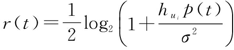
In this paper, we use Shannon’s capacity formula over an AWGN channel, and thus, the relationship between r(t) and p(t) for packet i is given by
(2)
where σ2 is the variance of the channel noise, and hui is the channel gain between the BS and the intended receiver of packet i. Thus, according to Eq.(2), we can write fi(·) as
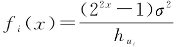
(3)
Hence, it can be easily verified that fi(·) is a convex and increasing function of the transmission rate.
For convenience, we refer the transmitter status with the transmission power p(t)>0 and that with p(t)=0 as “on” and “off” status. Hence, without loss of generality, we can assume the circuit power during the “on” and “off” status to be α>0 W and α=0 W because the circuit power in the “off” status is much smaller than that in the “on” status. Thus, the power consumption model considered in this paper is given by[12]
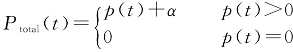
(4)
1.2 Problem formulation
For the general case involving multiple users, i.e. the downlink problem of cellular networks, the energy required to transmit packet i is denoted by fi(·), i∈{1,2,…,M}. Note that the transmission energy function fi(·) may be different for different packets as the receiver of each packet is not necessarily the same and therefore, each packet may undergo a different channel. An example to illustrate this is that the N receivers are not equidistant from the transmitter. Denote the transmission power at time t of packet i as
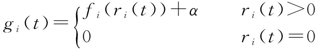
(5)
where ri(t) is the transmission rate of packet i at time t.
Thus, the problem of finding the optimal energy-efficient transmission schedule to minimize the total energy consumption can be formulated as
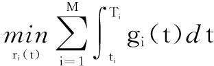
(6a)
s.t.![]() ∀i∈{1,2,…,M}
∀i∈{1,2,…,M}
(6b)
The above optimization is over ri(t) such that for any t, only one of ri(t) is non-zero. Based on the convexity of the function f(·), we have the following lemma.
Lemma 1 In the optimal transmission schedule, each packet should be transmitted at a constant rate.
The proof of Lemma 1 is similar to Ref.[5] and is thus omitted.
According to Lemma 1, each packet should be transmitted at a constant rate. Let r={r1,r2,…,rM} collect the constant transmission rates of all the packets. Due to the consideration of the non-ideal circuit power, i.e., α>0, it may be more energy efficient for the transmitter to be off for some periods of time[12]. Denote τi,off as the amount of time between the end of the transmission period of the i-th packet and the arrival time of the (i+1)-th packet. For example, if the (i+1)-th packet arrives when the i-th packet is still transmitting, τi,off will be equal to zero. Thus, the off-period τi,off can be calculated as
![]() ∀i
∀i
(7)
where τh is the transmission time of packet h.
We aim to find the optimal transmission strategy to minimize the total energy consumption of the M packets. Therefore, given Lemma 1, the original problem posed in (6) can be equivalently reformulated as
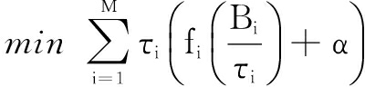
(8a)
s.t.![]() ∀i
∀i
(8b)
![]() ∀i
∀i
(8c)
where (8b) denotes the packet causality constraints, i.e., each packet transmission cannot begin before the packet arrives, and (8c) denotes the deadline constraints, i.e., packet i must be completely delivered before the deadline Ti.
To present the optimal offline schedule that solves the problem in (8), we expand previous results[3,5,7] on the case of ideal circuit power, i.e., α=0 to incorporate individual deadline constraints. Then, we propose an offline schedule for the case of α>0. Finally, we prove the optimality of our offline schedule.
2.1 Multi-packet case for the downlink problem with ideal circuit power
We consider the multi-packet case for the downlink problem with ideal circuit power, i.e., M≥1, α=0. A similar problem is studied in Ref.[7], where all packets have the same deadline. Regardless of individual deadline or the same deadline for the packets, we know that in the case of ideal circuit power, due to the monotonicity of the function fi, the most energy-efficient transmission scheme has no idling period, i.e., the optimal τi,off=0, for i=1,2,…,M.
For convenience, let
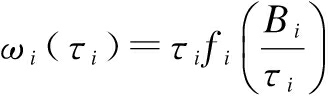
(9)
which denotes the transmission energy for packet i that takes transmission duration τi. Therefore, (8) is reformulated as
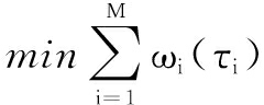
(10a)
s.t.![]() ∀i
∀i
(10b)
![]() ∀i
∀i
(10c)
It is observed in Ref.[7] that the cost function of the above problem is the sum of the convex energy functions and each energy function has its own constraint, allowing us to perform local optimization, which will satisfy the individual deadline constraint of each packet.
Based on the moveright algorithm in Ref.[7], we propose the individual deadline (ID) moveright algorithm that solves problem (10) and it is presented as below.
Algorithm 1 ID moveright algorithm

for i=1 to M do

end for
while flag=0 do

for i=1 to M-1 do

end for
if τk==τk-1 then
Set flag=1
end if
end while
In Algorithm 1, ![]() denotes that the time packet i starts to be transmitted in the k-th iteration, and
denotes that the time packet i starts to be transmitted in the k-th iteration, and ![]() denotes the transmission time of packet i in the k-th iteration. The key of the algorithm is to choose the transmission duration
denotes the transmission time of packet i in the k-th iteration. The key of the algorithm is to choose the transmission duration ![]() of packet i that minimizes the total energy of packet i and packet i+1, while the total transmission duration is fixed at
of packet i that minimizes the total energy of packet i and packet i+1, while the total transmission duration is fixed at ![]() ], i.e., the length of transmission time is
], i.e., the length of transmission time is ![]() . In the first iteration, fix
. In the first iteration, fix ![]() and
and ![]() , and move
, and move ![]() to the right (see Fig.1) to obtain
to the right (see Fig.1) to obtain ![]() , which satisfies
, which satisfies

(11)
where w1(·) and w2(·) are defined in Eq.(9). Compared with the result of Ref.[7], we add T1 into the constraint of the minimization of (11), because the starting time of the second packet cannot be later than the deadline of the first packet, otherwise, the schedule will be idle which cannot be optimal due to the decreasing
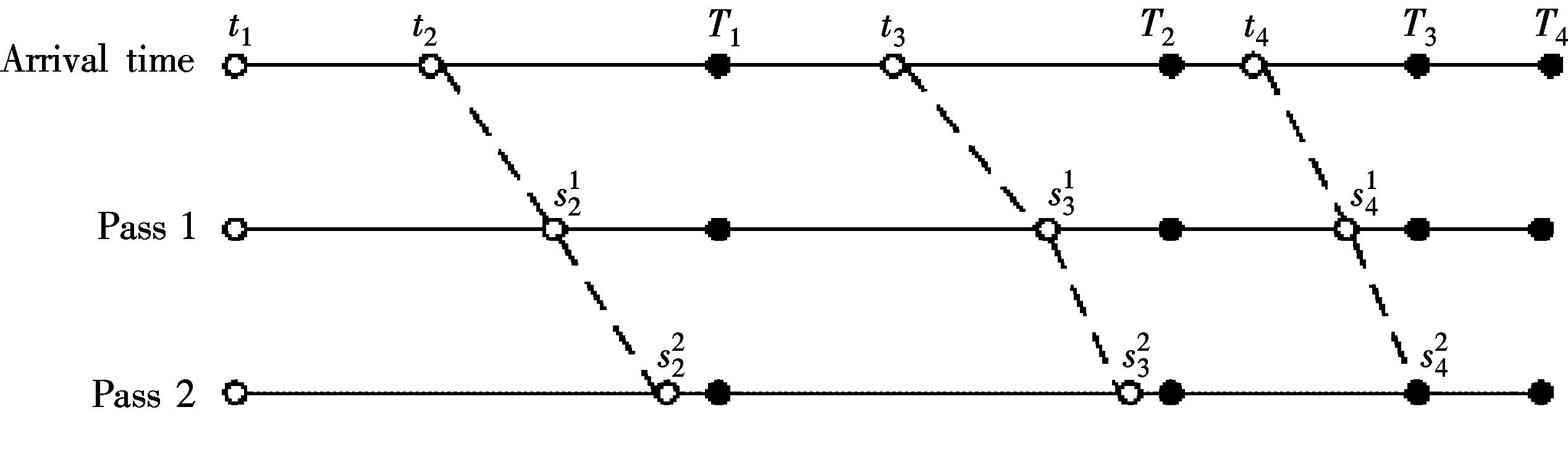
Fig.1 Illustration of ID moveright algorithm
nature of fi, i=1,2,…,M.
After we have obtained ![]() from (11), set
from (11), set ![]() . Continue to do this for every packet and this is counted as one iteration. After k iterations, if
. Continue to do this for every packet and this is counted as one iteration. After k iterations, if ![]() , then the algorithm converges and we obtain the transmission schedule of the M packets.
, then the algorithm converges and we obtain the transmission schedule of the M packets.
For the more general case, ![]() ,Ti]) returns
,Ti]) returns ![]() which satisfies
which satisfies

(12)
To solve Eq.(12), we denote the cost function of Eq.(12) as
g(x)
![]()
(13)
and note that g(x) is convex in x. The derivative of g(x) is given as
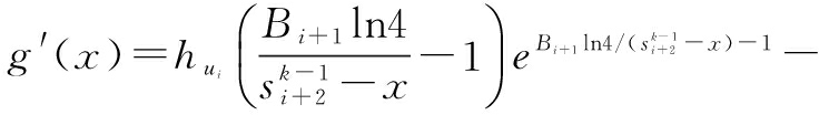

(14)
Let x* satisfy
g′(x*)=0
(15)
Since g(x) is a convex function, we know that such x* is unique. If ![]() }], then Algorithm 1 returns
}], then Algorithm 1 returns ![]() =x* and
=x* and ![]() will be moved right to
will be moved right to ![]() . If
. If ![]() , the packet transmission will be limited by the causality constraint and
, the packet transmission will be limited by the causality constraint and ![]() , which means that the transmission starting point of packet i+1 remains the same as that in the previous iteration.
, which means that the transmission starting point of packet i+1 remains the same as that in the previous iteration.
Note that the case ![]() } only occurs when
} only occurs when ![]() , since if
, since if ![]() ≤Ti, the optimal solution to (12) is
≤Ti, the optimal solution to (12) is ![]() , which means that packet i+1 has no time to transmit. Hence, if
, which means that packet i+1 has no time to transmit. Hence, if ![]() }, then
}, then ![]() =Ti, which means that packet i only finishes transmitting by its deadline Ti and packet i+1 will start its transmission at time Ti. Note that in future iterations, since the starting time of packet i+1 cannot be moved further right, there is no need to calculate
=Ti, which means that packet i only finishes transmitting by its deadline Ti and packet i+1 will start its transmission at time Ti. Note that in future iterations, since the starting time of packet i+1 cannot be moved further right, there is no need to calculate ![]() , for
, for ![]() >k, i.e.,
>k, i.e., ![]() =Ti, for all
=Ti, for all ![]() >k.
>k.
Now, denote the optimal start-time sequence and the optimal transmission duration sequence as ![]() } and
} and ![]() }, respectively. In the following, it is proved that the algorithm ID moveright results in
}, respectively. In the following, it is proved that the algorithm ID moveright results in ![]() }. We first argue that the algorithm ID moveright stops at the sequence
}. We first argue that the algorithm ID moveright stops at the sequence ![]() } and
} and ![]() }. We then show
}. We then show ![]() }.
}.
Theorem 1 The following statements hold.
1) ID moveright stops, and returns a sequence ![]() }.
}.
![]() }.
}.
Proof
1) Due to the causality constraint, during the iterations of the algorithm, the movement of the transmission starting time of all the packets is either to the right or remains unchanged. Therefore, ![]() is monotonically non-decreasing. Also, it is obviously bounded from
is monotonically non-decreasing. Also, it is obviously bounded from ![]() to
to ![]() ∀i=2,3,…,M. Hence, the sequence
∀i=2,3,…,M. Hence, the sequence ![]() converges as k→∞ for all i=1,2,…,M. Since
converges as k→∞ for all i=1,2,…,M. Since ![]() , the algorithm stops at the sequence
, the algorithm stops at the sequence ![]() }.
}.
2) Since the objective function in problem (10) is convex and all the constraints are linear, problem (10) is a standard convex problem and we will show that ![]() } satisfies the Karush-Kuhn-Tucker (KKT) conditions. First, according to the above discussion, it is clear that
} satisfies the Karush-Kuhn-Tucker (KKT) conditions. First, according to the above discussion, it is clear that ![]() } is a feasible solution since it satisfies the deadline constraint (10b) and the causality constraint (10c). Then, we only need to check that there are proper Lagrange multipliers specified by the KKT conditions. Let λi, γi, i=1,2,…,M denote the Lagrange multipliers associated with all the constraints. Hence, the Lagrangian function of (10) can be expressed as
} is a feasible solution since it satisfies the deadline constraint (10b) and the causality constraint (10c). Then, we only need to check that there are proper Lagrange multipliers specified by the KKT conditions. Let λi, γi, i=1,2,…,M denote the Lagrange multipliers associated with all the constraints. Hence, the Lagrangian function of (10) can be expressed as
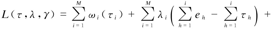
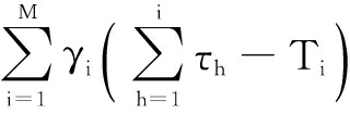
(16)
The KKT conditions can be obtained by differentiating L(τ,λ,γ) with respect to τi as
(17)
By subtracting the (m+1)-th equation from the m-th for ∀m=1,2,…,M-1, we obtain

(18)
where y(τm)=ωm(τm)+ωm+1(cm-τm) and y′(τ) is the first derivative of y(τ). Note that τm is the only variable since τm+τm+1 is a constant value cm for ∀m=1,2,…,M-1 in each iteration. Compared to Eq.(13), we find that the properties of y′(τm) are the same as those of g′(x) since x-sm=τm and sm+2-x=τm+1=c-τm.
Furthermore, the Lagrange multipliers λm and γm must satisfy the following KKT conditions:
(19a)

(19b)
Substituting ![]() for τm, we have the following three conditions.
for τm, we have the following three conditions.
 .
.
 ).
).
 ).
).
To sum up, we obtain λm≥0 and γm≥0, and we have the KKT conditions completely satisfied. This proves that ![]() } is the globally optimal solution
} is the globally optimal solution ![]() } of the problem (10).
} of the problem (10).
2.2 An offline schedule for general multi-packet case with non-ideal circuit power
We start with a simple case. Suppose that there is only a single packet, whose transmission rate is r1, to be transmitted to Receiver 1. In this case, the optimal transmission strategy can be formulated as
(20a)
s.t.![]()
(20b)
According to Ref.[13], the solution can be obtained as
(21)
in which

(22)
where W(·) is the Lambert W function, which is defined as
W(y)exp(W(y))=y
(23)
Thus, we obtain the following observations. If τee≥T1, we have ![]() =T1, then we know that there is no off-period, which means that the packet is transmitted as slowly as possible until its deadline, and this corresponds to an “always-on” transmission. If τee<T1, we have
=T1, then we know that there is no off-period, which means that the packet is transmitted as slowly as possible until its deadline, and this corresponds to an “always-on” transmission. If τee<T1, we have ![]() =τee, which means that the most energy-efficient way is to transmit at a rate of B1/τee until time τeeand the remaining period [τee,T1] is an off-period for the transmitter. To summarize, if τeedoes not violate the deadline constraint, then it is the most energy-efficient to transmit the packet using time τee. However, if τee violates the deadline constraint, then the transmission needs to use time smaller than τee. No transmission time larger than τee is optimal.
=τee, which means that the most energy-efficient way is to transmit at a rate of B1/τee until time τeeand the remaining period [τee,T1] is an off-period for the transmitter. To summarize, if τeedoes not violate the deadline constraint, then it is the most energy-efficient to transmit the packet using time τee. However, if τee violates the deadline constraint, then the transmission needs to use time smaller than τee. No transmission time larger than τee is optimal.
Similarly, for each packet i, i=1,2,…,M, denote τei as the EE transmission time of packet i, and it is defined as
(24)
Now, based on the above discussion, we propose the OOSCPMR (the optimal offline schedule with non-ideal circuit power for multi-receivers) algorithm. The key idea of the OOSCPMR algorithm is to find the “idle” periods of the transmitter as follows. First, let us define Scheme (i,k,t) as a transmission scheme of a consecutive sequence of packets, from packet i to packet k, where the starting time of the transmission is t and the duration of the transmission of packet j is τej, j=i,i+1,…,k, as defined in Eq.(24).
In the OOSCPMR algorithm,we start with the first iteration with packet 1 at time 0. We first find the index of the first packet, say packet k1, where subscript 1 denotes the first iteration, that satisfies Scheme (1,k1,0). Such index k1 can be written mathematically as
(25)
Next, we find the index of the first packet, say packet s1, where again subscript 1 denotes the first iteration, which satisfies the rule that Scheme (1,s1,0) violates the deadline constraint of packet s1. Such index s1 can be written mathematically as
(26)
If k1>s1, i.e., Scheme (1,k1,0) violates the deadline constraint of packet s1, then there should not be any idle periods for packet 1 to s1. Furthermore, the transmission schedule of packets 1 to s1 remains undetermined. If k1≤s1, i.e., Scheme (1,k1,0) does not violate the deadline constraints of packets 1 to k1, then the transmission scheme of packets 1 to k1 uses Scheme (1,k1,0), which means that there is an idle period from the end of the transmission time of packet k1 to the arrival time of packet k1+1, i.e., tk1+1. Furthermore, we repeat the above procedure for the second iteration starting from packet k1+1 at time tk1+1.
We repeat the above procedure for the second iteration starting from packet s1+1 at time Ts1. If we define m1=min(k1,s1), then we can see that, irrespective of the comparison of k1 and s1, the second iteration always starts with packet m1+1. If we further define
(27)
then, irrespective of the comparison between k1 and s1, the second iteration always starts at time tm1+1+q1.
Hence, we start the second iteration with packet m1+1 at time tm1+1+q1.
To describe more general scenario, we define

(28)

(29)
(30)
mj=min(kj,sj)
(31)
Thus, more generally, we start the j-th iteration with packet mj-1+1 at time tmj-1+1+qj-1. We first find the index of the first packet in Scheme (mj-1+1,kj,tmj-1+1+qj-1), which satisfies that the finish time of packet kj is before the arrival time of packet kj+1. For j>1, such index kj is written mathematically as in Eq.(28). Next, we find the index of the first packet, say packet sj, which satisfies that Scheme (mj-1+1,sj,tmj-1+1+qj-1) violates the deadline constraint of packet sj. For j>1, such index sj can be written mathematically as Eq.(29).
If kj>sj, i.e., Scheme (mj-1+1,kj,tmj-1+1+qj-1) violates the deadline constraint of packet sj, then the transmission schedule of packets mj-1+1 to sj contains no idle period. Furthermore, the transmission schedule of packets mj-1+1 to sj has not been determined.
If kj≤sj, i.e., Scheme (mj-1+1,kj,tmj-1+1+qj-1) does not violate the deadline constraints of packets mj-1+1 to kj, then the transmission scheme of packets mj-1+1 to kj uses Scheme (mj-1+1,kj,tmj-1+1+qj-1), which means that there is an idle period from the end of the transmission time of packet kj to the arrival time of packet kj+1, i.e., tkj+1. Furthermore, the transmission schedule of the unscheduled packets in the previous iterations, e.g. packets u1 and u2 (u1<u2), can be determined as follows: Let these packets be transmitted between time tu1 and tmj-1+1+qj-1 with no idle period and the ID moveright algorithm, i.e., Algorithm 1, can be used to find their transmission schedule. Then, we repeat the above procedure for the (j+1)-th iteration starting from packet kj+1 at time tkj+1. We repeat the above procedure until we reach TM.
Algorithm 2 OOSCPMR algorithm
1 Calculate τej according to Eq.(24).
2 Find kj and sj according to Eqs.(28) and (29), respectively.
3 Repeat step 2 until mj=M. Set J=min{j:mj=M} and l=1.
4 for j=1 to J do
if mj=kj then
Use Scheme (mj-1+1,kj,tmj-1+1+qj-1) for packets mj-1+1 to kj, i.e.,![]() .
.
if l>1 then
![]() .
.
end if
else
Set l=l+1
end if
end for
if kJ>sJ then
![]() ,M.
,M.
end if
2.3 Optimality of OOSCPMR algorithm
The next theorem states the optimality of the OOSCPMR algorithm.
Theorem 2 The OOSCPMR algorithm finds the optimal offline transmission schedule for Problem (8).
Proof Note that the calculation of (28) to (31) depends only on the attributes of the packets and does not depend on the transmission schedule of OOSCPMR. Thus, we may divide the M packets into two types:
1) Type Ⅰ packets
PⅠ![]() ,
,
i∈{1,2,…,M}}
(32)
These packets have been determined to be transmitted for the duration of τei, i∈PⅠ in OOSCPMR.
2) Type Ⅱ packets
![]() ,
,
i∈{1,2,…,M}}
(33)
The transmission schedule of these packets is determined by the ID moveright algorithm in OOSCPMR.
From the definition of τei in Eq.(24), we know that when the transmission schedule does not violate the causality or the deadline constraints, it is optimal to transmit the packets using τei. Type Ⅰ packets are the packets in the interval [mj-1+1,mj]. Since mj≤kj, we know that their causality constraints are not violated when transmitting at τei, i∈PⅠ, starting from instant tmj-1+1+qj-1. Furthermore, since mj≤sj, we know that their deadline constraints are not violated when transmitting at τei, i∈PⅠ, starting from instant tmj-1+1+qj-1. Thus, transmitting Type Ⅰ packets using the time of τei, i∈PⅠ is optimal, which is what OOSCPMR does.
As for Type Ⅱ packets, we only need to prove that there cannot be any idle periods in transmitting any of them. Since if there are no idle periods in transmitting them, then from Theorem 1, the ID moveright algorithm is optimal when there is no idle time, which is equivalent to the downlink problem with ideal circuit power discussed in Section 3.
So now, we prove that for Type Ⅱ packets, a scheme that has an idle period for packet i, for some i∈PⅡ, is suboptimal. We prove it by contradiction. Suppose that schedule N is optimal and it is feasible, and there is an idle period after the transmission of packet i, and the length of the idle period is ![]() . Denote the transmission time and the transmission start time of packet m as
. Denote the transmission time and the transmission start time of packet m as ![]() and
and ![]() , respectively, m=1,2,…,M. Then, according to the definition of Type Ⅱ packets, there exists some j such that i∈[mj-1+1,mj] where j satisfies kj>sj, i.e., mj=sj. According to Eq.(29), there must exist n∈{mj+1,…,mj+l-1} such that τn<τen. We can obtain the following two conditions.
, respectively, m=1,2,…,M. Then, according to the definition of Type Ⅱ packets, there exists some j such that i∈[mj-1+1,mj] where j satisfies kj>sj, i.e., mj=sj. According to Eq.(29), there must exist n∈{mj+1,…,mj+l-1} such that τn<τen. We can obtain the following two conditions.
1) If ![]() <τei, then we consider another transmission schedule
<τei, then we consider another transmission schedule ![]() +Δ for packet i, where Δ is small enough such that
+Δ for packet i, where Δ is small enough such that ![]() and τi′<τei. We can obtain that only the packet i changes the transmission time and it has been completely transmitted before deadline Ti by using the new transmission schedule. Thus, the new transmission schedule satisfies the deadline constraint. We also obtain that the new transmission schedule satisfies the causality constraint since the transmission start time of all the packets is the same as that of Schedule N. Thus, it is feasible. We know that the energy function is monotonously decreasing when τn<τen due to the pseudo-convex property, so the new transmission schedule will consume less energy. Therefore,
and τi′<τei. We can obtain that only the packet i changes the transmission time and it has been completely transmitted before deadline Ti by using the new transmission schedule. Thus, the new transmission schedule satisfies the deadline constraint. We also obtain that the new transmission schedule satisfies the causality constraint since the transmission start time of all the packets is the same as that of Schedule N. Thus, it is feasible. We know that the energy function is monotonously decreasing when τn<τen due to the pseudo-convex property, so the new transmission schedule will consume less energy. Therefore, ![]() is not the optimal solution. This condition leads to a contradiction.
is not the optimal solution. This condition leads to a contradiction.
2) If ![]() =τei, there must exist n∈{mj+1,…,i-1} such that τn<τen. Since if n∈{i+1,…,mj+l-1}, the transmission time of packet m is τem ∀m∈{i,…,mj+l-1}, which belongs to Type Ⅰ not Type Ⅱ. Thus, n∈{mj+1,…,i-1}. Now, we also consider another transmission schedule
=τei, there must exist n∈{mj+1,…,i-1} such that τn<τen. Since if n∈{i+1,…,mj+l-1}, the transmission time of packet m is τem ∀m∈{i,…,mj+l-1}, which belongs to Type Ⅰ not Type Ⅱ. Thus, n∈{mj+1,…,i-1}. Now, we also consider another transmission schedule ![]() +Δ for packet n and the idle period of packet i is
+Δ for packet n and the idle period of packet i is ![]() -Δ, where Δ is small enough such that
-Δ, where Δ is small enough such that ![]() and τn′<τen and
and τn′<τen and ![]() +Δ≤Tn. Thus, we can obtain that packet i can be completely transmitted before deadline Ti by using the new transmission schedule and the packet i+1 also starts to be transmitted at time
+Δ≤Tn. Thus, we can obtain that packet i can be completely transmitted before deadline Ti by using the new transmission schedule and the packet i+1 also starts to be transmitted at time ![]() and the transmission time of packets after packet i is the same as that of Schedule N. Thus, the new transmission schedule satisfies the deadline constraint. We also obtain that the new transmission schedule satisfies the causality constraint since the transmission start time si′ for i∈{n+1,i} of the new transmission schedule becomes greater than
and the transmission time of packets after packet i is the same as that of Schedule N. Thus, the new transmission schedule satisfies the deadline constraint. We also obtain that the new transmission schedule satisfies the causality constraint since the transmission start time si′ for i∈{n+1,i} of the new transmission schedule becomes greater than ![]() and other transmission start time is the same as that of Schedule N. Therefore, it is feasible. In a similar way, the new transmission schedule also consumes less energy. Then,
and other transmission start time is the same as that of Schedule N. Therefore, it is feasible. In a similar way, the new transmission schedule also consumes less energy. Then, ![]() is not the optimal solution. This condition also leads to a contradiction.
is not the optimal solution. This condition also leads to a contradiction.
In conclusion, there cannot be any idle periods for Type Ⅱ packets. From the above discussion, Theorem 2 is proved.
2.4 Computational complexity of OOSCPMR algorithm
The first step of the OOSCPMR algorithm is to find the value of J where J=min{j: mj=M} by means of a quick sort algorithm whose computational complexity is O(Mlog2M). The second step is to find the optimal transmission duration of each packet whose computational complexity is O(J). Thus, the computational complexity of the OOSCPMR algorithm is O(Mlog2M)+O(J).
To obtain the benchmark, we develop the optimal offline schedule by assuming complete information including the size, arrival time, deadline constraint of the packets during the time interval [0,T], which is an ideal situation. Thus, this provides a lower bound on the consumed energy in practical scenarios, where the future packet’s arrival information is not available. Furthermore, based on the optimal offline schedule, we can develop an online schedule that needs no future arrival information.
To better understand the online schedule, we first assume that there are N packets with different deadlines arriving at the buffer at a certain time t. Denote Bi and Ti, i=1,2,…,M as the size and the deadline instant of the i-th packet, respectively. Note that no new packet arrivals at the transmitter’s buffer. At the moment, we know the complete information of all the packets. According to the information, we use the above-mentioned optimal offline schedule algorithm to find the optimal transmission duration. Next, we extend the unified arrival case to the general arrival case, i.e., there are new packets arriving at the buffer.
To be specific, when the first packet with its deadline T1 arrives at the transmitter’s buffer at t=0, we schedule the first packet by applying the OOSCPMR algorithm according to its arrival information until the second packet arrives. When the second packet arrives at the transmitter’s buffer at ta,2, there is the residue of packet 1 with its deadline T1 and the newly arrived packet 2 with its own deadline T2 in the buffer if the first packet has not been completely transmitted at ta,2. We take ta,2 as the new starting point, and according to the packets in the buffer at ta,2, we run the OOSCPMR algorithm and start transmitting. We repeat the above procedure when a packet arrives. In summary, when a packet arrives, we restart the OOSCPMR algorithm according to the packets in the buffer at that time.
In this section, we compare our proposed policy with the existing policies by numerical simulations. The existing policies in Ref.[5] are obtained by using a calculus approach and an appealing “string visualization” is provided for the optimal policy.
We consider that there are 5 types of channel gain ![]() ={1,2,3,4,5} and the AWGN noise σ2=1, which can lead to 5 types of energy functions. The bandwidth W=1 kHz and the circuit power α=3 W. First, we generate the packet sequence with a Poisson arrival rate of λ=0.1,0.2,…,0.9,1 packet/s during the time window [0,80] s. Each packet’s deadline is set to be 1 s and each packet’s size is set to be 1 kbit. Each packet has one energy function chosen from a set of 5 types uniformly at random.
={1,2,3,4,5} and the AWGN noise σ2=1, which can lead to 5 types of energy functions. The bandwidth W=1 kHz and the circuit power α=3 W. First, we generate the packet sequence with a Poisson arrival rate of λ=0.1,0.2,…,0.9,1 packet/s during the time window [0,80] s. Each packet’s deadline is set to be 1 s and each packet’s size is set to be 1 kbit. Each packet has one energy function chosen from a set of 5 types uniformly at random.
Fig.2 presents the average total energy consumption between our proposed policies and the existing policies in Ref.[5] with different packet arrival rates. It is observed that the proposed online schedule has similar performance to the optimal offline policy which has a lower bound performance and our proposed policies outperform the other two policies proposed in Ref.[5]. It is also observed that the energy consumption always increases as λ increases and this is because the total size of packets will increase with the increase of the packet’s arrival rate. Also, note that the energy consumption increases sharply from 0.4 to 0.5 packet/s since many packets are transmitted for the time of τei. However, at λ>0.5 packet/s, very few packets can satisfy the deadline constraints when transmitting data for the time of τei, and the transmitter is almost always on.

Fig.2 Performance comparison of energy consumption with different arrival rates of the packets
Next, we consider a total number of 500 packets within the time window [0,500] s averaged over 1 000 independent simulations.
Fig.3 shows the average total energy consumption of our proposed policies and the existing policies in Ref.[5] with different packet deadline constraints. Again, the proposed optimal offline policy gives a lower bound performance to the proposed online policy, and our proposed policies always outperform those of Ref.[5]. It is also observed that the total energy consumption first decreases and then remains unchanged as the deadline constraints become looser. This is because when the deadline constraint is sufficiently loose, all packets should be transmitted for the duration of τei, and any transmission time larger than τei will only increase the energy consumption.
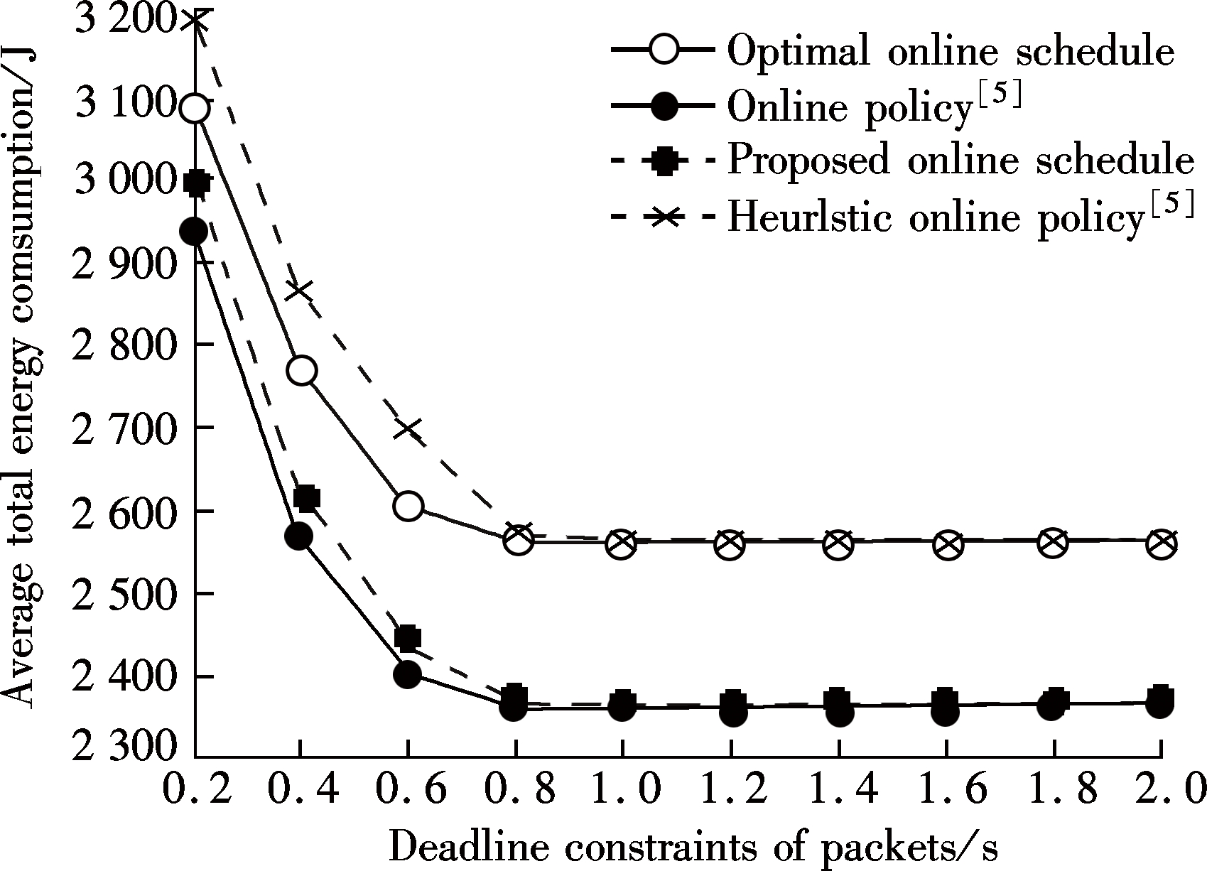
Fig.3 Performance comparison of energy consumption with different life time durations of packet
We have investigated a wireless network over an AWGN channel with non-ideal circuit power involving a single transmitter and multiple receivers. We propose a novel OOSCPMR algorithm to find the optimal offline solutions to minimize the total energy consumed including the transmission energy and the circuit energy. It is shown that, the packets can be divided into two types, where one type of packet is determined to be transmitted using the EE transmission time, and the other type of packet is determined by the ID moveright algorithm, which is the most energy-efficient transmission schedule with ideal circuit power. According to the proposed optimal offline schedule, the development of an energy-efficient online schedule is also discussed.
[1]Ephremides A. Energy concerns in wireless networks[J]. IEEE Wireless Communications, 2002, 9(4): 48-59.DOI:10.1109/mwc.2002.1028877.
[2]Hasan Z, Boostanimehr H, Bhargava V K. Green cellular networks: A survey, some research issues and challenges[J]. IEEE Communications Surveys & Tutorials, 2011, 13(4): 524-540. DOI:10.1109/SURV.2011.092311.00031.
[3]Uysal-Biyikoglu E, Prabhakar B, El Gamal A. Energy-efficient packet transmission over a wireless link[J]. IEEE/ACM Transactions on Networking, 2002, 10(4): 487-499. DOI:10.1109/tnet.2002.801419.
[4]Jin Y, Xu J, Qiu L. Energy-efficient scheduling with individual packet delay constraints and non-ideal circuit power[J]. Journal of Communications and Networks, 2014, 16(1): 36-44. DOI:10.1109/jcn.2014.000007.
[5]Zafer M A, Modiano E. A calculus approach to energy-efficient data transmission with quality-of-service constraints[J]. IEEE/ACM Transactions on Networking, 2009, 17(3): 898-911. DOI:10.1109/tnet.2009.2020831.
[6]Lee J, Jindal N. Energy-efficient scheduling of delay constrained traffic over fading channels[J]. IEEE Transactions on Wireless Communications, 2009, 8(4): 1866-1875. DOI:10.1109/t-wc.2008.080037.
[7]El Gamal A, Nair C,Prabhakar B, et al. Energy-efficient scheduling of packet transmission over wireless networks[C]//Proceedings of IEEE Twenty-First Annual Joint Conference of the IEEE Computer and Communications Societies. 2002: 1773-1782.
[8]Blume O, Eckhardt H, Klein S, et al. Energy savings in mobile networks based on adaptation to traffic statistics[J]. Bell Labs Technical Journal, 2010, 15(2): 77-94. DOI:10.1002/bltj.20442.
[9]Jin Y, Xu J, Qiu L. Energy-efficient scheduling with individual packet delay constraints and non-ideal circuit power[J]. Journal of Communications and Networks, 2014, 16(1): 36-44. DOI:10.1109/jcn.2014.000007.
[10]Zheng N,Chen T Y, Wang X,et al. Energy-efficient transmission schedule for delay-limited bursty data arrivals under non-ideal circuit power consumption[J]. IEEE Transactions on Vehicular Technology, 2016, 65(8): 6588-6600.
[11]Chen W, Neely M J, Mitra U. Energy-efficient transmissions with individual packet delay constraints[J]. IEEE Transactions on Information Theory, 2008, 54(5): 2090-2109. DOI:10.1109/tit.2008.920344.
[12]Xu J, Zhang R. Throughput optimal policies for energy harvesting wireless transmitters with non-ideal circuitpower[J]. IEEE Journal on Selected Areas in Communications, 2012, 32(2): 322-332.
[13]Jin Y, Xu J, Qiu L. Energy-efficient scheduling with individual packet delay constraints and non-ideal circuit power[J]. Journal of Communications and Networks, 2014, 16(1): 36-44. DOI:10.1109/jcn.2014.000007.
References:
摘要:在考虑非理想电路损耗情况下,研究了无线网络下行链路中一个发送端和多个接收端的最优传输调度策略问题.根据该问题特殊的结构,提出了新颖的OOSCPMR(非理想电路损耗下有多个接收端的最优离线调度)算法,从而找到使得传输能效最优的离线调度策略.被传输的包分为2种类型:类型Ⅰ可以利用高能效的传输时间来进行传输,类型Ⅱ要使用ID moveright 算法来确定其传输时间.最后,根据提出的OOSCPMR算法,提出了实际可行的在线调度算法.仿真结果表明,最优离线传输调度是在线传输调度的下界,且提出的调度算法的性能优于其他现有的调度算法.
关键词:能量效率;传输调度;多接收端;非理想电路功耗
中图分类号:TN929.53
Foundation items:The National Natural Science Foundation of China(No.61571123, 61521061), the National Science and Technology Major Project(No.2016ZX03001011-005), the Research Fund of National Mobile Communications Research Laboratory of Southeast University(No.2017A03), Qing Lan Project.
Citation::Yang Zhuoqi, Zhou Qing, Liu Nan, et al. Energy-efficient data transmission with non-ideal circuit power for downlink cellular networks[J].Journal of Southeast University (English Edition),2017,33(1):5-13.
DOI:10.3969/j.issn.1003-7985.2017.01.002.
DOI:10.3969/j.issn.1003-7985.2017.01.002
Received 2016-08-26.
Biographies:Yang Zhuoqi(1991—), female, master; Liu Nan(corresponding author), female, doctor, professor, nanliu@seu.edu.cn.