Abstract:To study the effect of speed on the biomechanics of a knee joint during running, a biomechanical model of human lower limb joints is established based on the Kane method and semi-physical simulation. Experiments on the running process were made at different speeds for healthy young men. The influence of running speed on knee joint motion is analyzed quantitatively and a mathematical model of the knee angle is established with speed as the independent variable. Results show that, at the moment of the heel contacting with the ground, with the increase of speed, the calf stretches forward more, and the calf and thigh are closer to the same line. In the middle stage of a gait cycle, the thigh stretches back, and then the calf and thigh are close to collineation. At that moment, the stretch of the posterior cruciate ligament is the largest, and the slower the speed, the more obvious the collineation. The maximal joint angle of the calf relative to the thigh appears in the later stage, and the maximal joint angle increases with the increase of the velocity. With the increase of the running speed, the phase of the curve of knee angle moves forward. The results can be used in the field of rehabilitation robotics and humanoid robot.
Key words:biomechanics; knee joint; mathematical model; speed; joint torque
Human biomechanics has been one of the important research fields for many years[1-4]. Recently, many studies on how environment affects the human movement function are carried out[5-7]. As one of the lower limb joints, the knee joint plays an important function during running. During running, the velocity is one of the most important parameters, which not only has an influence on the speed of movement, but has an effect on the characteristics of the joint motion and the kinetics of the joint[8-11]. In this article, the influence of the running speed on the biomechanics of the knee joint is studied. The results are important for the understanding of human movement and provide important data and methods for the application in the fields of rehabilitation robotics and humanoid robots[11-15].
A gait cycle is composed of support phase and swing phase. It is defined as the period that the same heel contacts with the ground sequentially twice. In this article, the left human lower extremity is taken as a reference, and the moment of the left heel contacting the ground is defined as the starting point of the gait cycle.
The flexion and extension of the knee joint refer to the knee movement along the coronal axis. In accordance with international practice, the knee angle is defined as the intersection angle of the calf and the thigh in the coronal axis. The Kane method is used to establish the dynamic model of the swing and the support phase during running.
The definition of the body coordinate system is shown in Fig.1. In Fig.1, B is the trunk, H, K and A are the hip joint, knee joint and ankle joint, respectively. H is the origin of the fixed coordinate system. The hip angle θh is defined as the angle between the thigh and the vertical axis. The knee angle θk is defined as the angle between the calf and the extended line of the thigh. The ankle angle θa is defined as the angle between the foot and the vertical line of the calf. The angles between xi andxo are taken as generalized coordinates. βi is the internal coordinate which is defined as βi=θi-θi-1(i=2,3). i, j, k are the base vectors that represent horizontal axis x, vertical axis y, and axis z which is perpendicular to paper surface outward, respectively. The velocity vi of each particle in the system is expressed as the pseudo velocity ur, that is, partial velocity. ![]() , the coefficient of ur, can be called the r partial velocity of particle i.
, the coefficient of ur, can be called the r partial velocity of particle i.

Fig.1 Coordinate system
The lower extremity dynamic model for the swing phase is shown in Fig.2. l1 is the thigh length, and l2 is the calf length. F1, F2 and F3 represent the gravity acting on the thigh, calf and foot, respectively. M1, M2, and M3 are the torque of the hip joint, knee joint and foot. ![]() ,
, ![]() 2 and
2 and ![]() represent the torques relative to the thigh, calf and the centroid of the foot, respectively.
represent the torques relative to the thigh, calf and the centroid of the foot, respectively. ![]() ,
, ![]() and
and ![]() are the inertia forces acting on the thigh, calf and foot, respectively.
are the inertia forces acting on the thigh, calf and foot, respectively. ![]() ,
, ![]() and
and ![]() are the inertia moments relative to the thigh, calf and the centroid of the foot. The generalized inertia force Kane equations for the human lower extremity are derived as follows:
are the inertia moments relative to the thigh, calf and the centroid of the foot. The generalized inertia force Kane equations for the human lower extremity are derived as follows:


m2gl1sinθ1-m3gl1sinθ1
(1)


0
(2)


(3)
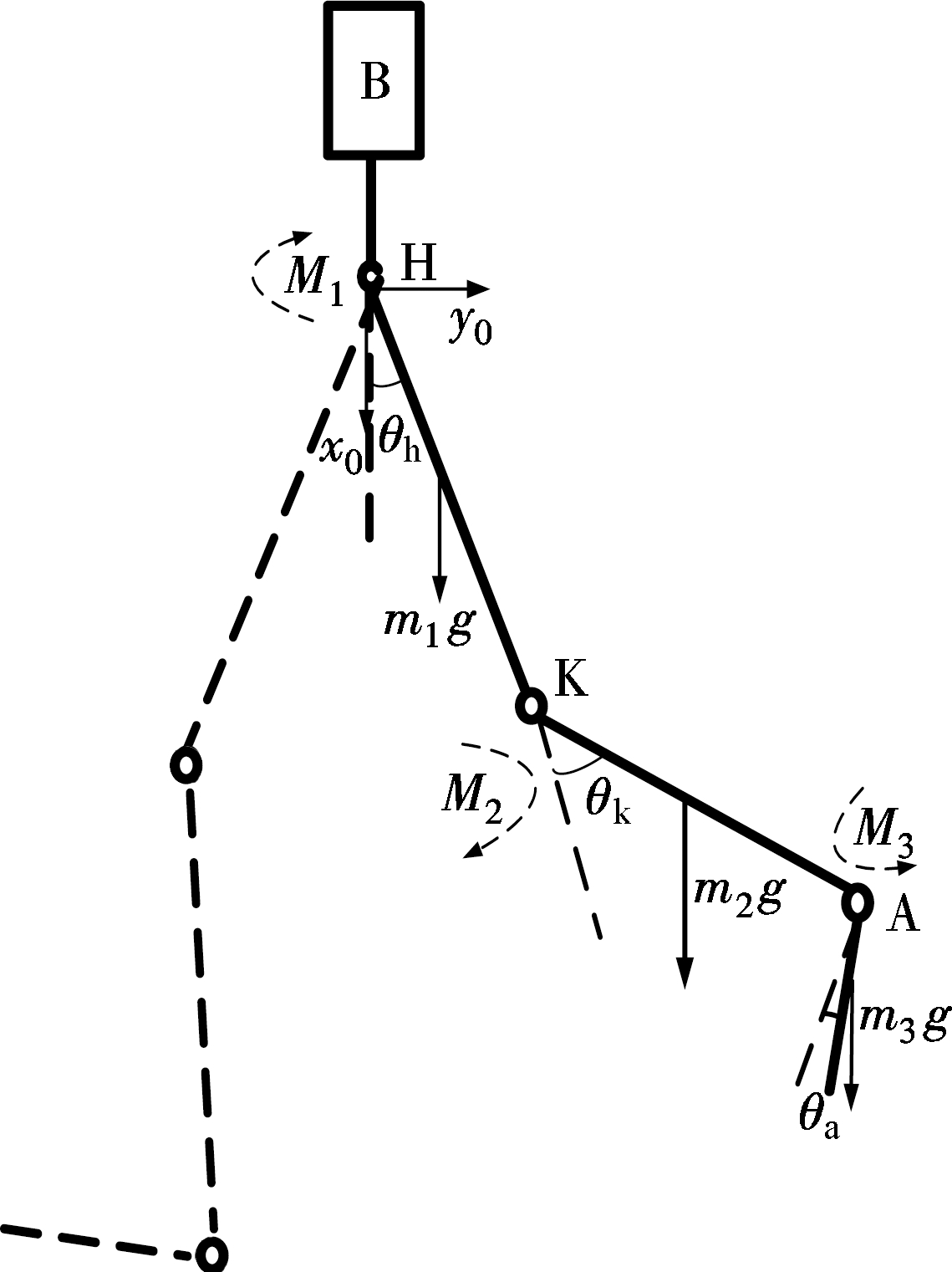
Fig.2 Dynamic model of unilateral lower extremity
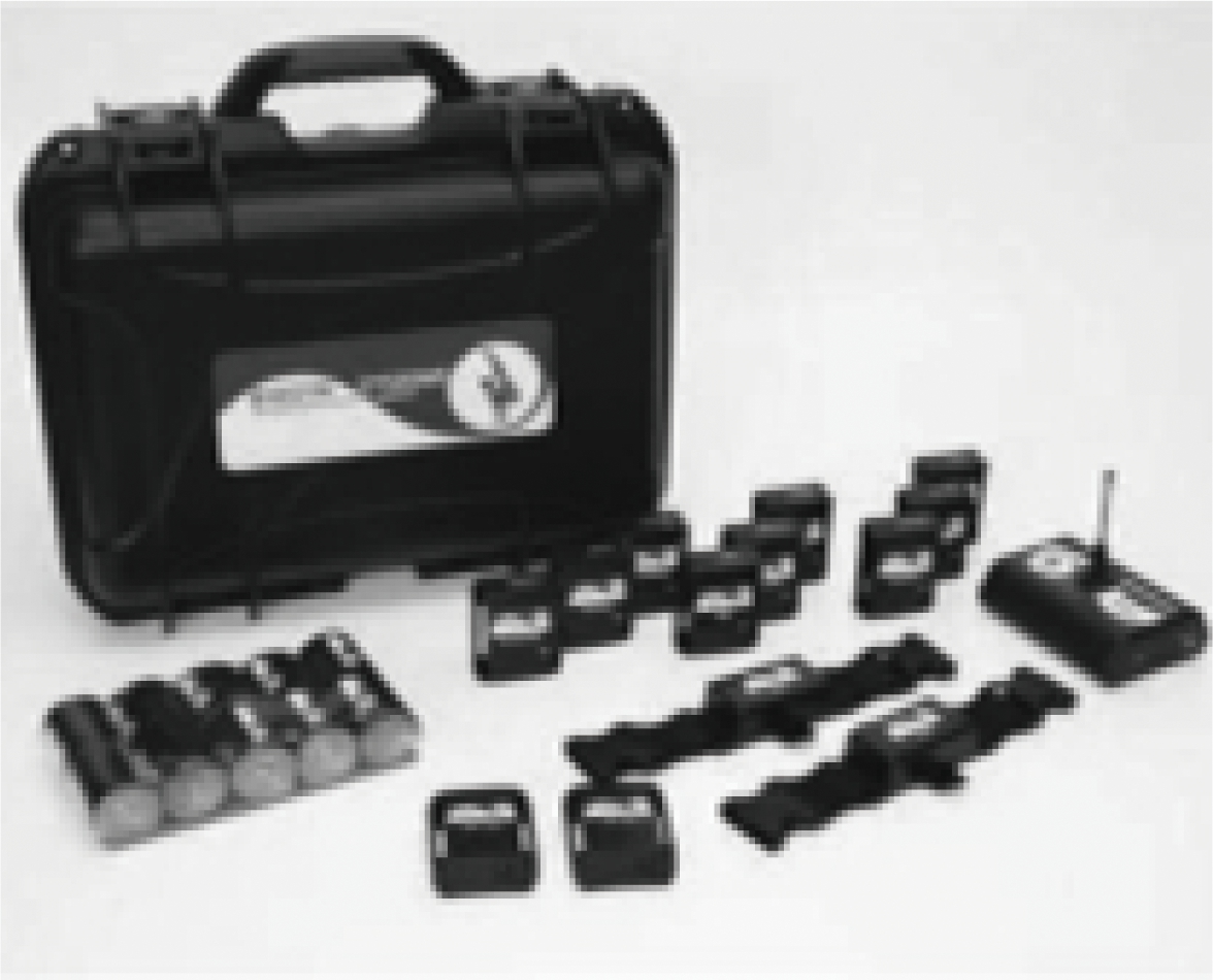
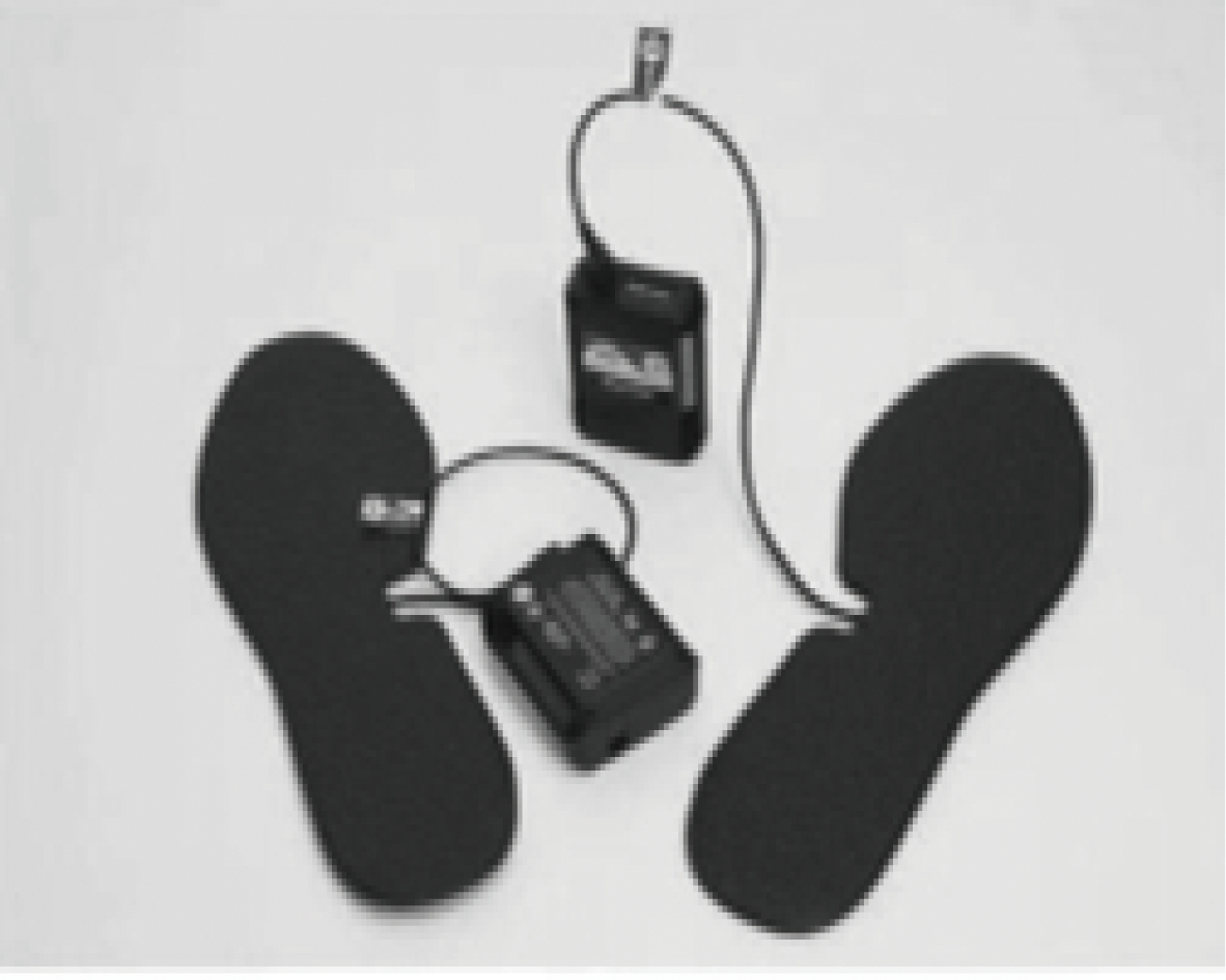
The functional assessment biomechanics system(FAB)developed by the Canadian NEODYN company and a wireless gait phase detection system are applied in this research (see Fig.3). The sampling frequency is 100 Hz. These systems can capture the human dynamic motion information by using the multi-information fusion algorithm. The systems have advantages such as high precision, small volume, convenient wear, wireless transmission which can collect walking data indoors and outdoors.
(a)
(b)
Fig.3 Experimental installation. (a) Functional assessment of biomechanics system; (b) Wireless gait analysis detection system
In our experiment, 20 healthy young men (height 170 to 183 cm, weight 50 to 90 kg, age 20 to 30) are randomly selected as subjects. These subjects run on the treadmill at different speeds from 4 to 12 km/h. The effective data acquisition time for each speed is 30 s. To avoid errors caused by maladjustment, treadmill running training should be performed before experiments. The experimental process is shown in Fig.4.
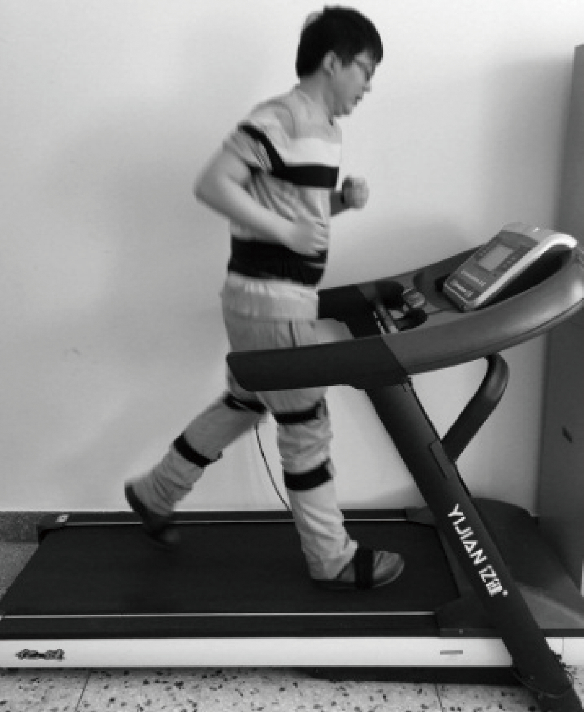
Fig.4 The experimental process of running on the treadmill
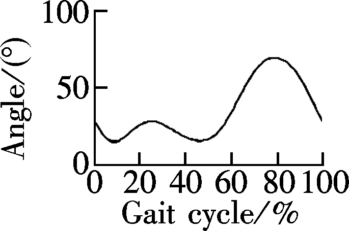
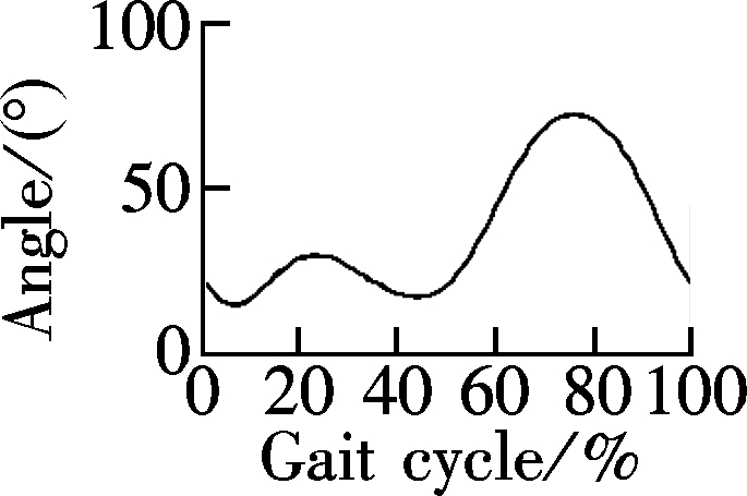
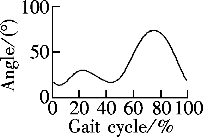
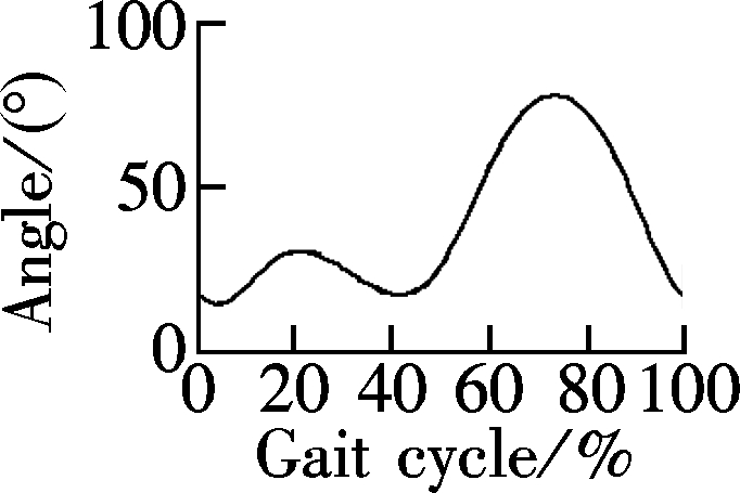
A sample (weight 67 kg, height 181 cm) who runs at 12 km/h is selected. The original data of the knee angle (period for 30 s) is shown in Fig.5. The experimental curve in a single gait cycle is obtained after data processing(see Fig.6). The irregular curves (see Fig.6) result from the nonstandard actions of experimental subjects. Fig.7 shows the average knee angle curve in a gait cycle (The abnormal curve in Fig.6 is removed). To make the data more universal, Fig.8 shows the curves of the average experimental data of single cycle of the knee joint obtained from 20 samples who run at different speeds (v) from 4 to 12 km/h.

Fig.5 The original data curve
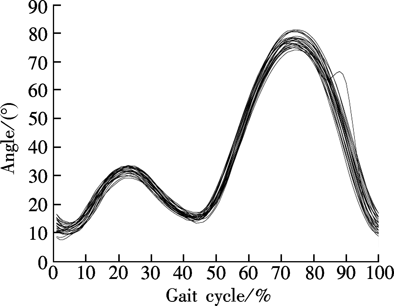
Fig.6 The knee angle curves of a sample running at 12 km/h
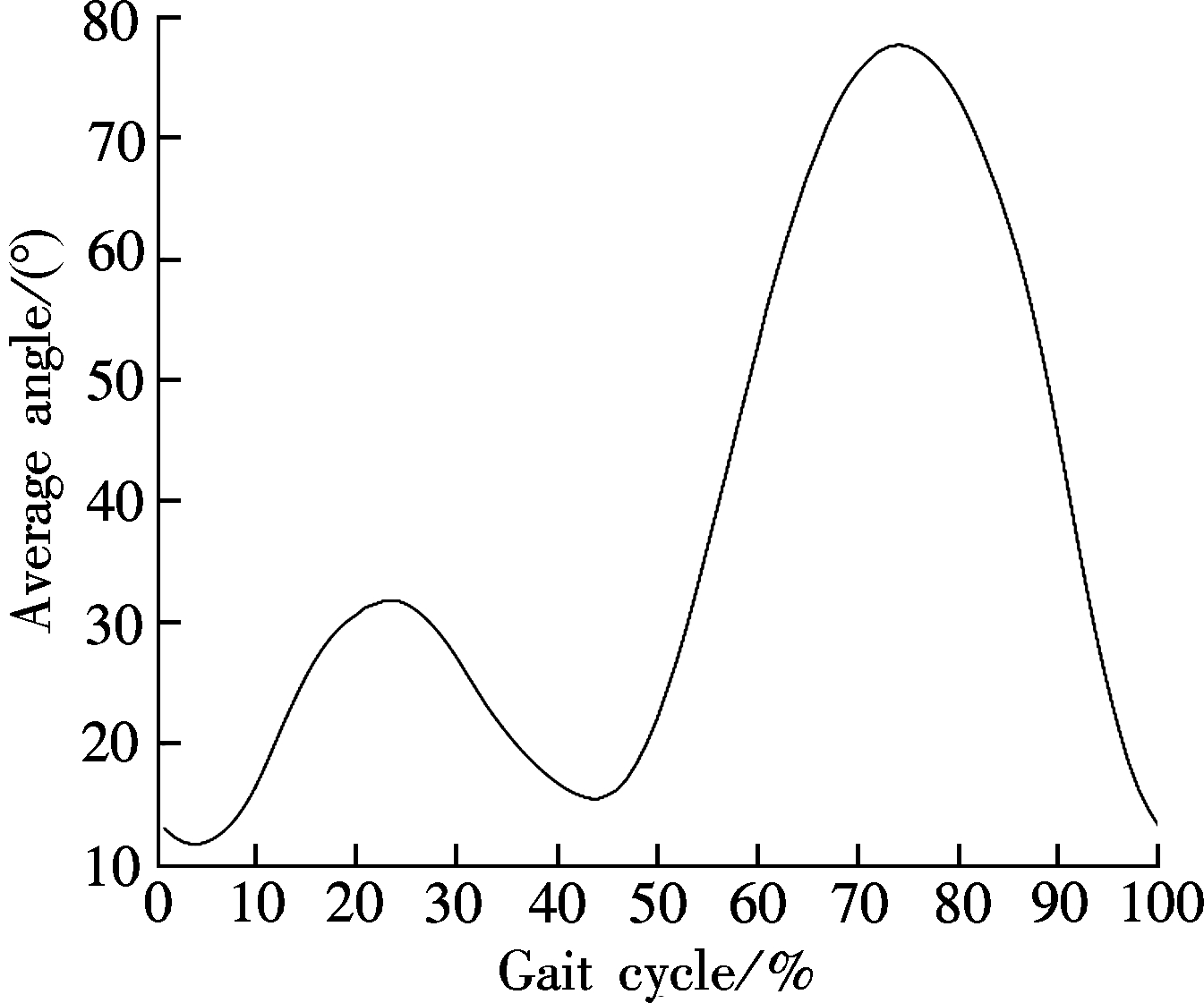
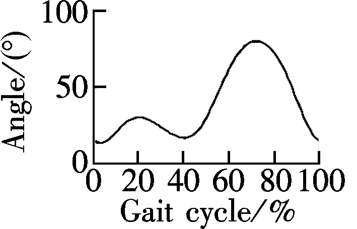
Fig.7 The knee angle curve in a cycle
According to the above experimental results, the following conclusions can be obtained:
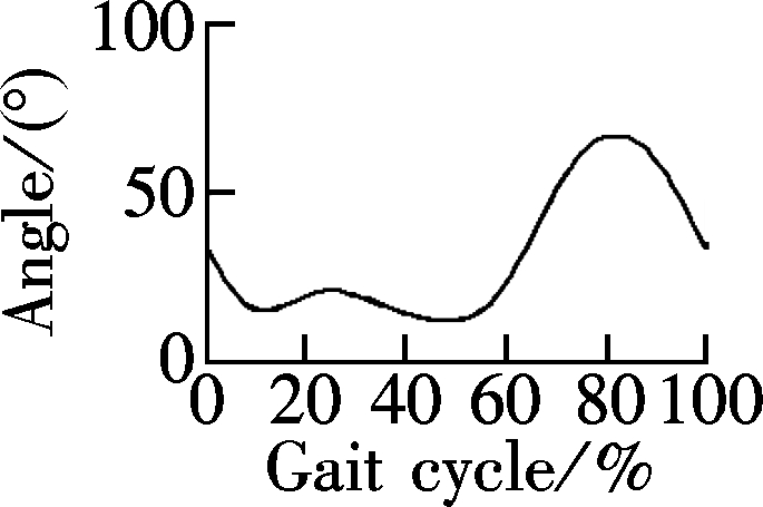
1) In the early stage of a gait cycle (the heel contacting the ground), the knee angle for different velocities first decreases slightly and then increases slightly, with the minimum angle greater than 0°. With the decrease of the running speed, the knee angle will increase at the moment of the heel contacting with the ground. As the speed increases, the knee angle of the heel point contacting with the ground will decrease. At the moment of the heel contacting with the ground, the more the calf stretches forward, the closer to the same line the calf and thigh are.
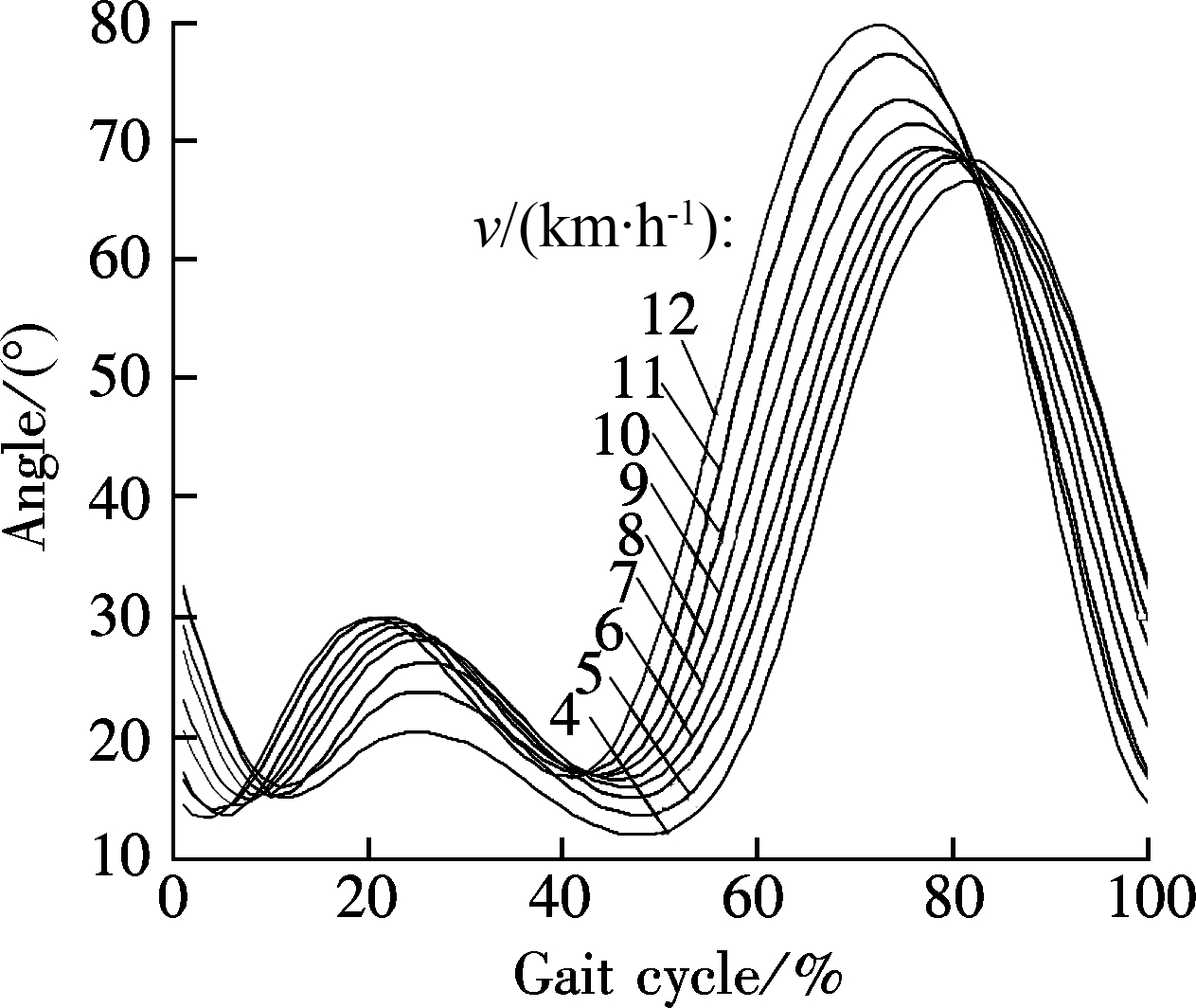
Fig.8 The mean curves of knee angle for twenty samples at different speeds (4 to 12 km/h)
2) In the middle stage of a gait cycle (the contralateral heel contacting the ground), the knee angle first decreases and then increases. When the second trough appears, the thigh stretches back to the greatest degree, and the calf and thigh are close to collineation. Now, the stretch of the posterior cruciate ligament is the largest, but the minimum value is still greater than 0°, which means that no collineation occurs. The slower the speed, the more obvious the collineation.
3) In the later stage of a gait cycle, the knee joint has an obvious buckling process, forming a biggish wave crest. The maximal joint intersection angle of the calf and the thigh appears from this stage. The maximal joint angle increases with the increase of the velocity.
4) The effect of the speed on the phase can be obtained from Fig.8. With the increase of the running speed, the phase of the curve of the knee angle moves forward.
The knee angle curve is fitted with the Fourier function, and the mathematical model of the knee angle is established as
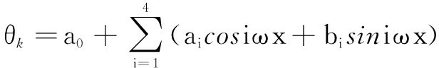
(4)
where the independent variable x is the percentage period of a gait cycle; a0, ai, bi and ω are fitting coefficients. Tab.1 shows the fitting function coefficients and the goodness of fit of the knee angle curve at different speeds.
The goodness of fit is close to 1. Therefore, the above functions can be used to characterize the knee angle during running. To further study the influence of speed on the knee joint motion, the regression equation is constructed with the speed as the independent variable and the fitting coefficient as the dependent variable. The results are
Tab.1 The fitting curve coefficients and goodness of the knee joint angle at different speeds
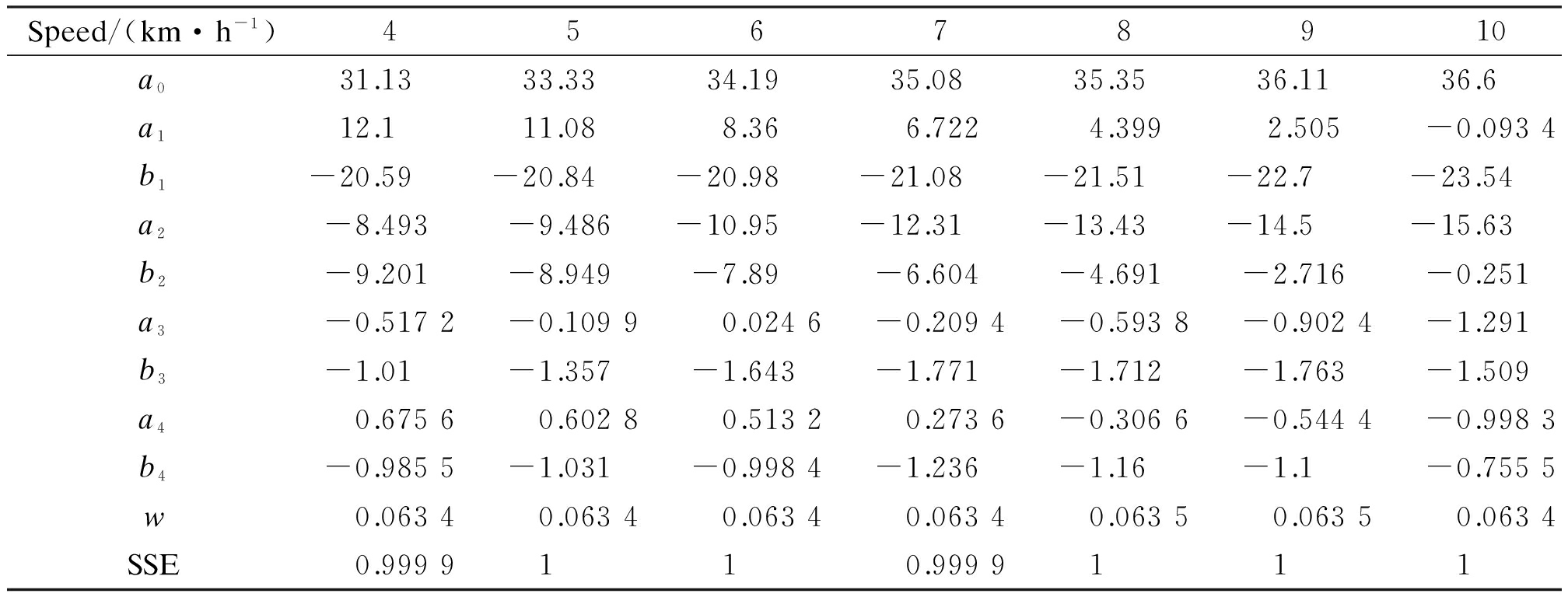
Speed/(km·h-1)456789101112a0 31.13 33.33 34.19 35.08 35.35 36.11 36.6 38.25 38.96a1 12.1 11.08 8.36 6.722 4.399 2.505-0.0934-1.775-4.731b1-20.59-20.84-20.98-21.08-21.51-22.7-23.54-25.46-26.61a2-8.493-9.486-10.95-12.31-13.43-14.5-15.63-15.95-15.86b2-9.201-8.949-7.89-6.604-4.691-2.716-0.251 2.163 5.054a3-0.5172-0.1099 0.0246-0.2094-0.5938-0.9024-1.291-1.603-2.021b3-1.01-1.357-1.643-1.771-1.712-1.763-1.509-1.472-1.281a4 0.6756 0.6028 0.5132 0.2736-0.3066-0.5444-0.9983-1.233-1.276b4-0.9855-1.031-0.9984-1.236-1.16-1.1-0.7555-0.4584 0.1019w 0.0634 0.0634 0.0634 0.0634 0.0635 0.0635 0.0634 0.0634 0.0633SSE 0.9999 1 1 0.9999 1 1 1 1 0.9999
given as follows:
a0=0.029v3-0.720v2+6.457v+15.130
(5)
a1=0.002v3-0.087v2-1.099v+18
(6)
a2=0.019v3-0.374v2+1.096v-8.085
(7)
a3=0.011v3-0.303v2+2.432v-6.053
(8)
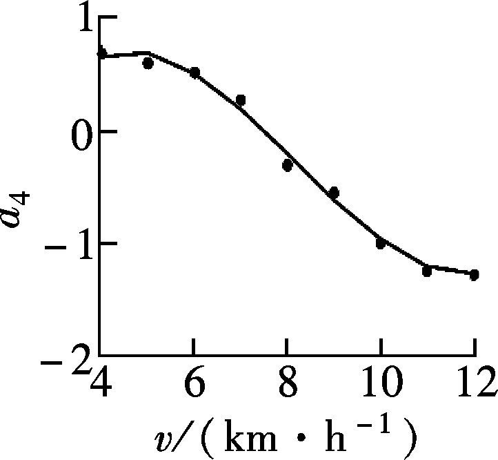
a4=0.011v3-0.261v2+1.731v-2.785
(9)
b1=-0.003 4v3-0.042v2+0.629v-22.340 (10)
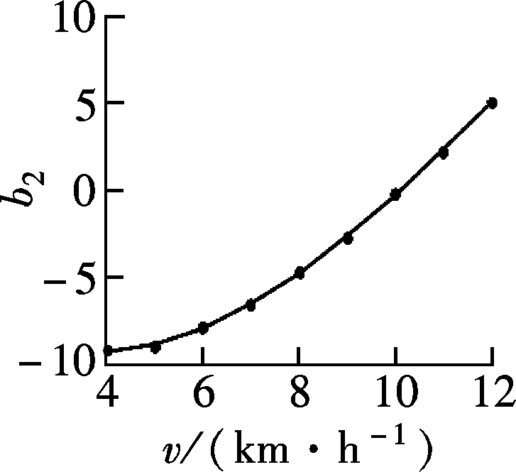
β2=-0.011v3+0.419v2-2.735v-4.339
(11)
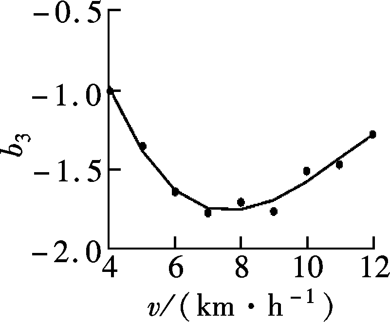
b3=-0.004v3+0.136v2-1.364v+2.548
(12)
b4=0.006v3-0.093v2+0.425v-1.549
(13)
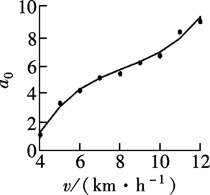
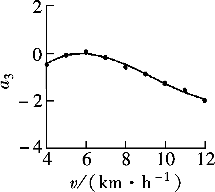
The fitting curves are shown in Fig.9.
(a)

(b)

(c)
(d)
(e)

(f)
(g)
(h)

(i)
Fig.9 The fitting coefficients of the model of the knee angle. (a) a0; (b) a1; (c) a2; (d) a3; (e) a4; (f) b1; (g) b2; (h) b3; (i) b4
Since the speed variance has little influence on ω, the value of 0.063 4 is taken as the average value. The mathematical model of the knee angle can be acquired by substituting Eqs.(5) to (13) and ω into Eq.(4). f(v) is a function with the speed v as the independent variable. Fig.10 shows the experimental curves and the derived model curves, and these two types of curves are almost the same. Thus, the established mathematical model f(v) conforms with the movement of the knee angle. It also accords with the influence of the speed on the knee joint motion.
(a)

(b)

(c)
(d)

(e)
(f)
(g)
(h)
(i)
Fig.10 The experimental result and the derived model result at different speeds. (a) v=4 km/h; (b) v=5 km/h; (c) v=6 km/h; (d) v=7 km/h; (e) v=8 km/h; (f) v=9 km/h; (g) v=10 km/h; (h) v=11 km/h; (i) v=12 km/h
The above method can also be applied to deduce the mathematical model of the hip and ankle angles. By introducing the mathematical models of the hip, knee and ankle into the biomechanical Kane equations of the lower extremity, the analytic expressions of the hip, knee and ankle torques of the lower limb which vary with the running speed can be acquired, and the theoretical curve can be acquired.
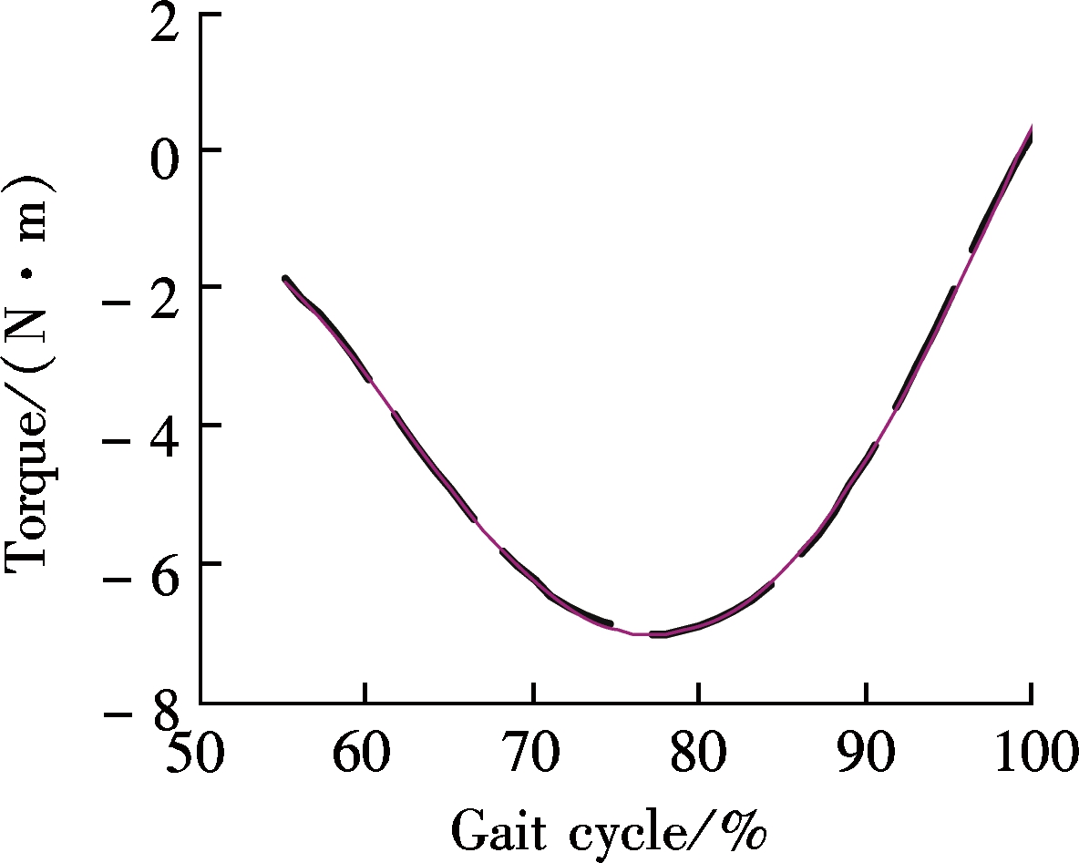
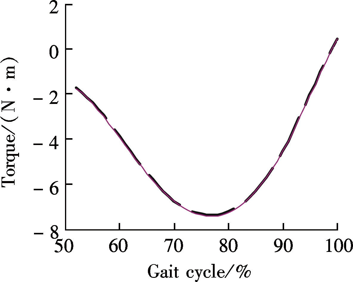
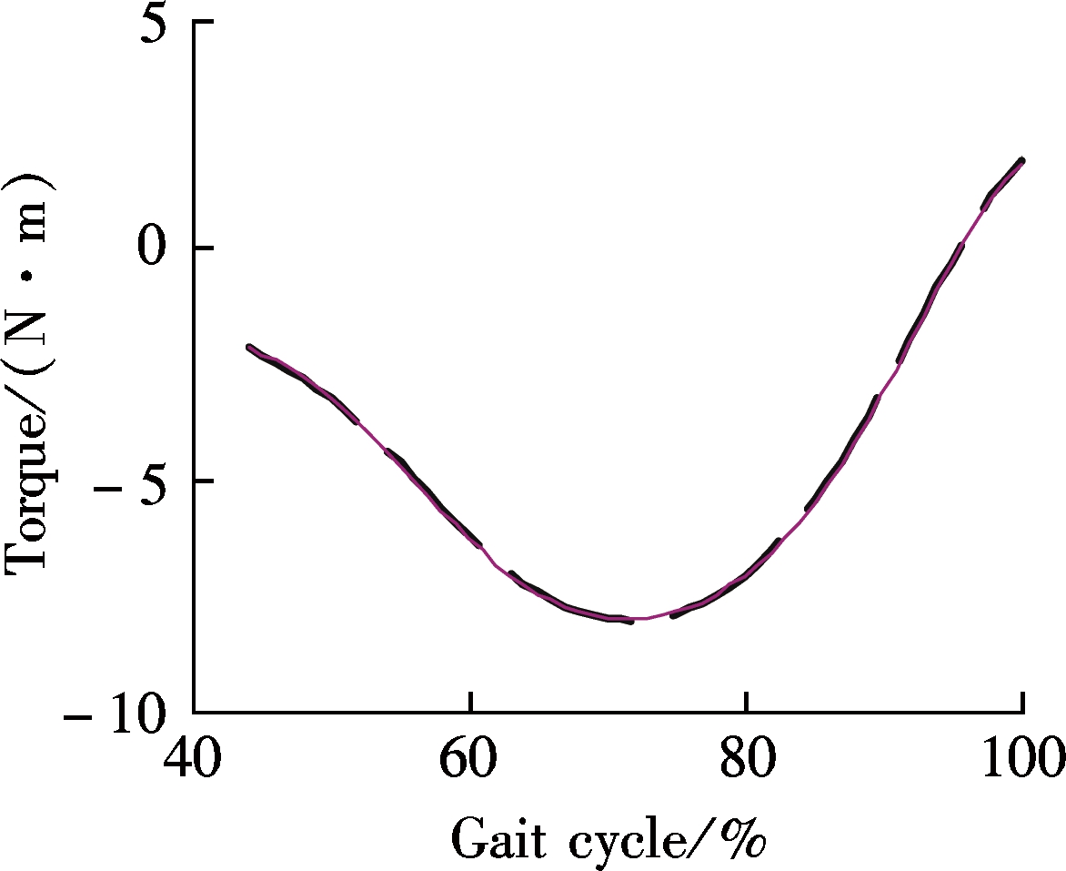
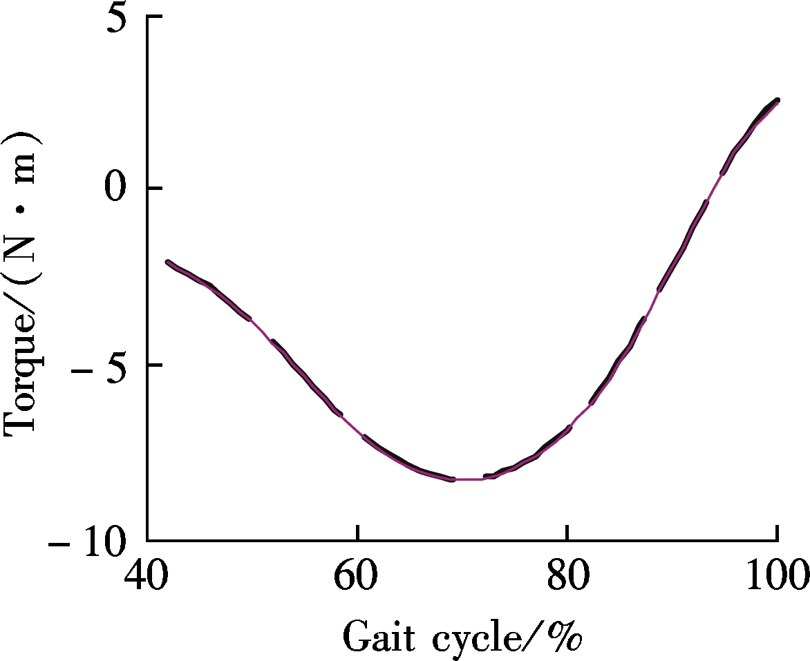
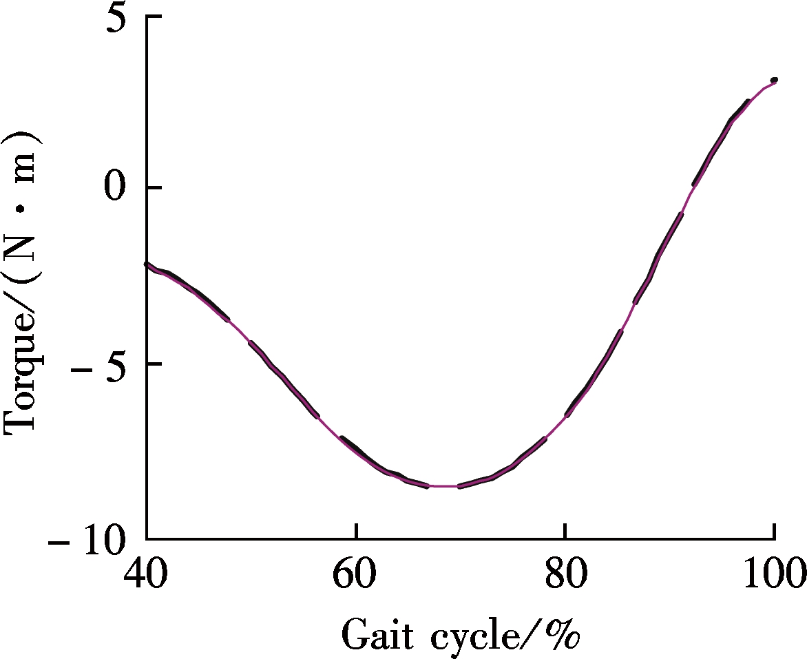
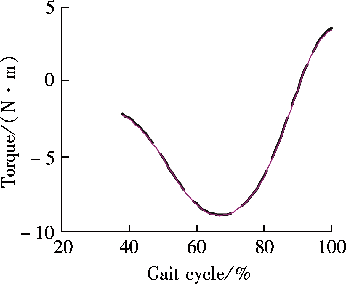
The biomechanical model of the human lower extremity is established by using the SimMechanics toolbox of Matlab. The measured data of the hip, knee and ankle angles are used as the inputs of the model. To conduct the simulation, the body inertia parameters such as height, weight and inertia are given in the model. The simulation results of the knee torque of the swing period are obtained. The theoretical knee torque is obtained by deducing from the mathematical model of knee angle and the kinetic Kane equation of the lower extremity motion. It can be seen from Fig.11 that the two types of curves coincide with each other approximately.
(a)
(b)
(c)

(d)
(e)
(f)
(g)
(h)

(i)
![]()
Fig.11 The simulation results and theoretical results of the knee torque in the swing period. (a) v=4 km/h; (b) v=5 km/h; (c) v=6 km/h; (d) v=7 km/h; (e) v=8 km/h; (f) v=9 km/h; (g) v=10 km/h; (h) v=11 km/h; (i) v=12 km/h
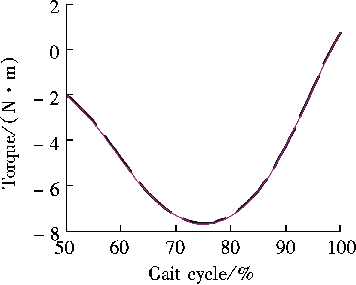
The accuracy of the kinetic equation of the human lower extremity which is constructed by the Kane equation can be verified. Also, the accuracy of the mathematical model of the joint angle based on speed can be verified. The average knee torque for 10 samples is acquired by applying the above method, as shown in Fig.12. It can be seen that the amplitude of the knee torque of the swing phase increases with the increases of the speed, and the phase of the curve of knee angle moves forward.
The biomechanical model of the knee joint is developed.
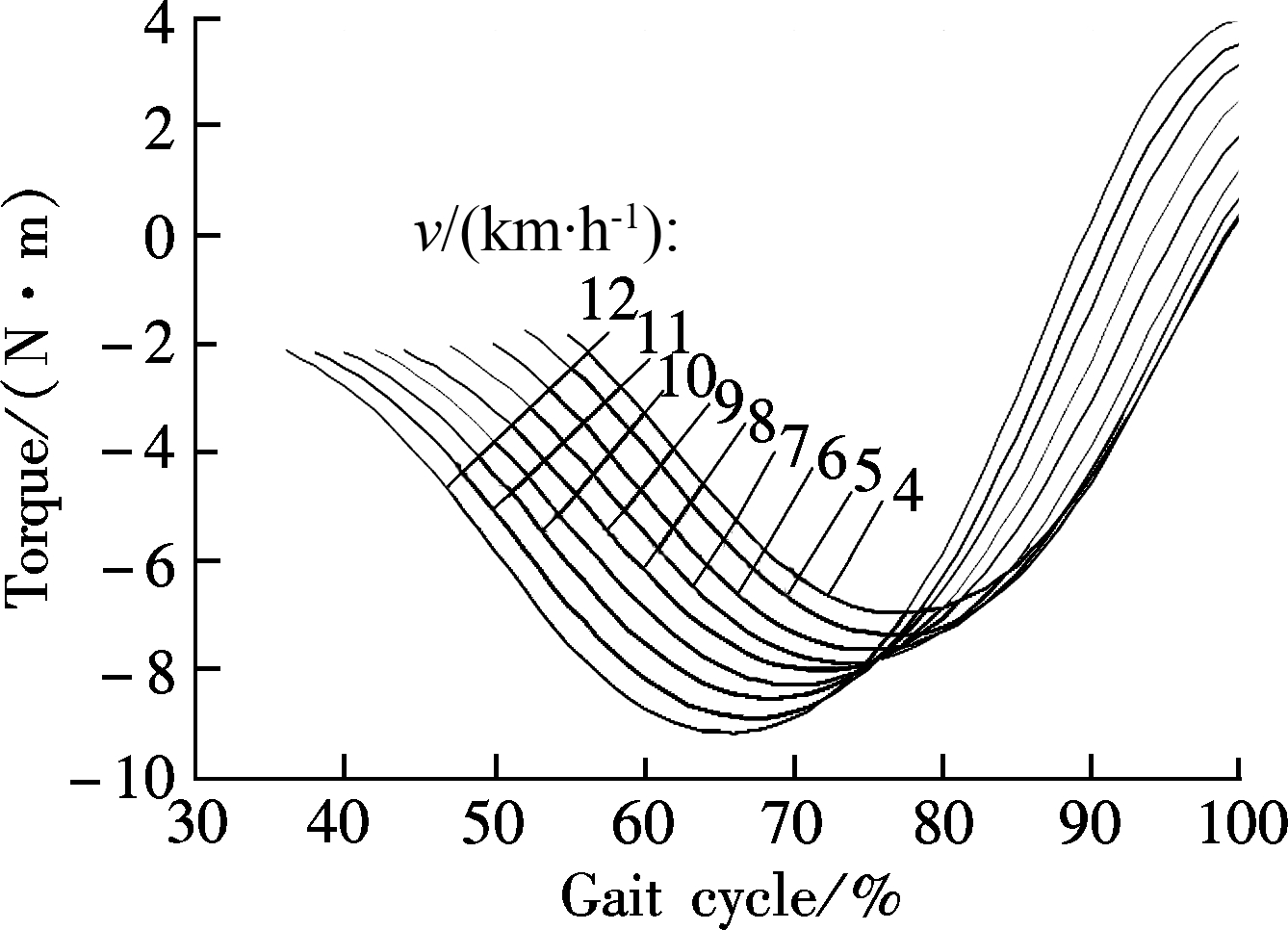
Fig.12 The mean curves of the knee torque for multiple samples at different speeds (4 to 12 km/h)
The running process of healthy young men at different speeds is tested. The influence of running speed on the knee joint motion is analyzed quantitatively, and a mathematical model of the knee angle is established, in which the speed is an independent variable. Based on the semi-physical simulation, the accuracy of the biomechanical model of lower extremity and the mathematical model of the knee joint angle are verified. The method can be extended to the study of the hip and ankle biomechanics. The experimental data and relevant conclusions can provide reference for rehabilitation robotics, astronaut training and sports research.
[1]Lu T W, Chang C F. Biomechanics of human movement and its clinical applications[J]. Kaohsiung Journal of Medical Sciences, 2012, 28(sup): S13-S25. DOI: 10.1016/j.kjms.2011.08.004.
[2]Zhang Y L, Ma Z J, Yu X. Relationship analysis of treadmill slope and knee motion mechanics [J]. Journal of Mudanjiang Teachers College (Natural Science Edition), 2011(1): 52-54. (in Chinese)
[3]Li J W, Li X W, Chen C C. Analysis of sport parameters of human on running machine[J]. Modern Computer, 2012(7): 10-14. (in Chinese)
[4]Salim M S, Maknoh F N, Omar N, et al. A biomechanical analysis of walking and running on a treadmill in different level of inclined surfaces[C]//International Conference on Biomedical Engineering. Perlis, Malaysia, 2012: 308-312.
[5]Yabe Y, Watanabe H, Taga G. Treadmill experience alters treadmill effects on perceived visual motion[J]. PLoS ONE, 2011, 6(7): e21642. DOI: 10.1371/journal.pone.0021642.
[6]Bartels W, Demol J, Gelaude F, et al. Computed tomography-based joint locations affect calculation of joint moments during gait when compared to scaling approaches[J]. Computer Methods in Biomechanics and Biomedical Engineering, 2015, 18(11): 1238-1251. DOI:10.1080/10255842.2014.890186.
[7]Wang L J. Research on rehabilitative robot prototype and gait control[D]. Harbin: College of Mechanical and Electrical Engineering, Harbin Engineering University, 2010: 17-19. (in Chinese)
[8]Piazza S J, Baxter J R, Celik H. Joint morphology and its relation to function in elite sprinters[J]. Procedia IUTAM, 2011, 2: 168-175. DOI: 10.1016/j.piutam.2011.04.017.
[9]Mijailovic N, Vulovic R, Milankovic I, et al. Assessment of knee cartilage stress distribution and deformation using motion capture system and wearable sensors for force ratio detection[J]. Computational and Mathematical Methods in Medicine, 2015, 2015: 963746. DOI:10.1155/2015/963746.
[10]Slawinski J, Bonnefoy A, Ontanon G, et al. Segment-interaction in sprint start: Analysis of 3D angular velocity and kinetic energy in elite sprinters[J]. Journal of Biomechanics, 2010, 43(8): 1494-1502. DOI: 10.1016/j.jbiomech.2010.01.044.
[11]Wu Z J,Zhao Z H,Tang L. SVM-based method for real time classification of pedestrian gait[J]. Electronic Measurement Technology, 2015, 38(7): 41-44. (in Chinese)
[12]Xiao F, Liu A M, Wu Y, et al. Comparison of biomechanical characteristics of the knee joint during forward walking and backward walking[J]. Journal of Medical Biomechanics, 2015, 30(3): 264-269. (in Chinese)
[13]Yang S Z, Laudanski A, Li Q G. Inertial sensors in estimating walking speed and inclination: An evaluation of sensor error models[J]. Medical & Biological Engineering & Computing, 2012, 50(4): 383-393. DOI:10.1007/s11517-012-0887-7.
[14]Yang X J,Li C L,Xia Y, et al. Design of a new gait acquisition system on the treadmill[J]. Chinese Journal of Sensors and Actuators, 2012, 25(6): 751-755. (in Chinese)
[15]Hamon A, Aoustin Y, Caro S. Two walking gaits for a planar bipedal robot equipped with a four-bar mechanism for the knee joint[J]. Multibody System Dynamics, 2013, 31(3): 283-307. DOI:10.1007/s11044-013-9382-7.
References:
摘要:为了研究人在跑步过程中速度对膝关节运动生物力学的影响规律,基于Kane方法和半物理仿真方法建立下肢动力学模型,以健康男性青年为对象,对不同速度下的跑步过程进行实验研究和数据分析,建立以速度为自变量的膝关节运动模型.研究结果表明:步态初期足跟落地时刻,跑步速度越快,小腿向前伸展程度越大,越接近与大腿共线;步态中期,大腿向后伸展,小腿与大腿接近共线的最大程度,此时膝关节背面的韧带拉伸量最大,并且速度越慢,共线程度越明显;膝关节最大屈曲过程出现在步态后期,并且最大角度随着速度的增加而增加;随着跑步速度的增加,膝关节曲线前移.实验结论可用于康复机器人、类人机器人等研究领域.
关键词:运动生物力学;膝关节;数学模型;速度;关节力矩
中图分类号:TB18
Foundation items:The National Natural Science Foundation of China (No.51405095), the Fundamental Research Funds for the Central Universities (No.HEUCF160706), the Technological Innovation Talent Special Fund of Harbin (No.2014RFQXJ037).
Citation::Zhao Lingyan, Ma Xiaohao, Zhang Bingzao, et al. Biomechanical research of knee joint during the process of running[J].Journal of Southeast University (English Edition),2017,33(1):27-32.
DOI:10.3969/j.issn.1003-7985.2017.01.005.
DOI:10.3969/j.issn.1003-7985.2017.01.005
Received 2016-07-08.
Biography:Zhao Lingyan (1981—), female, doctor, lecturer, zly6668837@163.com.