Fig.1 Diagram of the proposed positioning methodology
Abstract:To address the problem that a general augmented state Kalman filter or a two-stage Kalman filter cannot achieve satisfactory positioning performance when facing uncertain noise of the micro-electro-mechanical system (MEMS) inertial sensors, a novel interacting multiple model-based two-stage Kalman filter (IMM-TSKF) is proposed to adapt to the uncertain inertial sensor noise. Three bias filters are developed based on different noise characteristics to cover a wide range of noise levels. Then, an accurate estimation of biases is calculated by the interacting multiple model algorithm to correct the bias-free filter. Thus, the vehicle positioning system can achieve good performance when suffering from uncertain inertial sensor noise. The experimental results indicate that the average position error of the proposed IMM-TSKF is 25% lower than that of the general TSKF.
Key words:interacting multiple model (IMM); two-stage filter; uncertain noise; vehicle positioning
The last two decades have witnessed an increasing trend in using integrated INS/GPS systems for vehicle positioning. Kalman filtering is traditionally used to fuse the information from both INS and GPS. In order to employ INS in mass-market applications, the industry has been directed toward using the micro-electro-mechanical system (MEMS) based INS. However, in a number of practical situations, the uncertain noise of MEMS INS may seriously degrade the performance of the filter or even cause the filter to diverge[1]. A general approach to solve this problem is to treat the noise variables as parts of the system state and then estimate them together with it. This will lead to an augmented state filter whose implementation can be computationally intensive. To maintain the computational cost at a lower level, the idea of using a two-stage filter to implement an augmented state filter was introduced[1]. The idea is to decouple the augmented filter into two parallel reduced-order filters. The first filter, the bias-free filter, is based on the assumption that the noise of MEMS inertial sensors is non-existant and the state vector is only comprised of navigation parameters (i.e., position, velocity, attitude, or their errors). The second filter, the bias filter, produces an estimation of the bias vector, which is composed of noise variables. The output of the first filter is then corrected with the output of the second filter.
It is well known that the successful use of the Kalman filter is greatly restricted by the strict requirements on a priori statistics information of the process and measurement noises[2]. These are specified in the form of process noise and measurement noise covariances, i.e. matrix Q and matrix R, respectively. Usually, the specification of matrix R can be directly derived from the accuracy characteristics of the measurement device. Meanwhile, the specification of Q is often attempted in a trial-and-error approach and considered to be constant[3]. However, due to the high uncertainty of the inertial sensor noise, the covariances of accelerometer biases and gyro drifts are difficult to determine and the specification of constant covariances might not be sufficient to provide an accurate filter performance. The adaptive KF (AKF) is one of the strategies to improve the estimation of the covariance matrices based on innovation. Usually, the AKF adjusts the covariance matrices through scale factors[4-5]. The major problem is that it is very difficult to choose an optimal scale factor. Even small changes in the scale factor may greatly affect filtering performance.
Over the past few years, the interacting multiple model (IMM)-based methods have been applied to vehicle positioning[6-7]. In these studies, the possible vehicle driving patterns are represented by a set of models, which are generally established according to different maneuvering or driving conditions. The IMM algorithm is used to calculate a weighted sum of the individual estimates from each model[8]. In our research, its capability to represent the noise behavior with different levels has been found to be useful to obtain more precise bias estimation.
In this paper, we aim at developing a novel vehicle positioning methodology which can adapt to uncertain inertial sensor noise. A structural adaptation approach based on the IMM algorithm provides a soft switching between the filters with different Q matrices, which indicates different noise levels. Moreover, the structure of the two-stage filter makes it possible to only adjust the filter involved with accelerometer biases and gyro drifts. Thus, the computational load can be reduced to a large extent. The proposed IMM-based two-stage Kalman filter (IMM-TSKF) can significantly improve the robustness of the vehicle positioning system when facing uncertain inertial sensor noise. The performance comparison between the proposed IMM-TSKF methodology and a general two-stage Kalman filter (TSKF) approach is demonstrated.
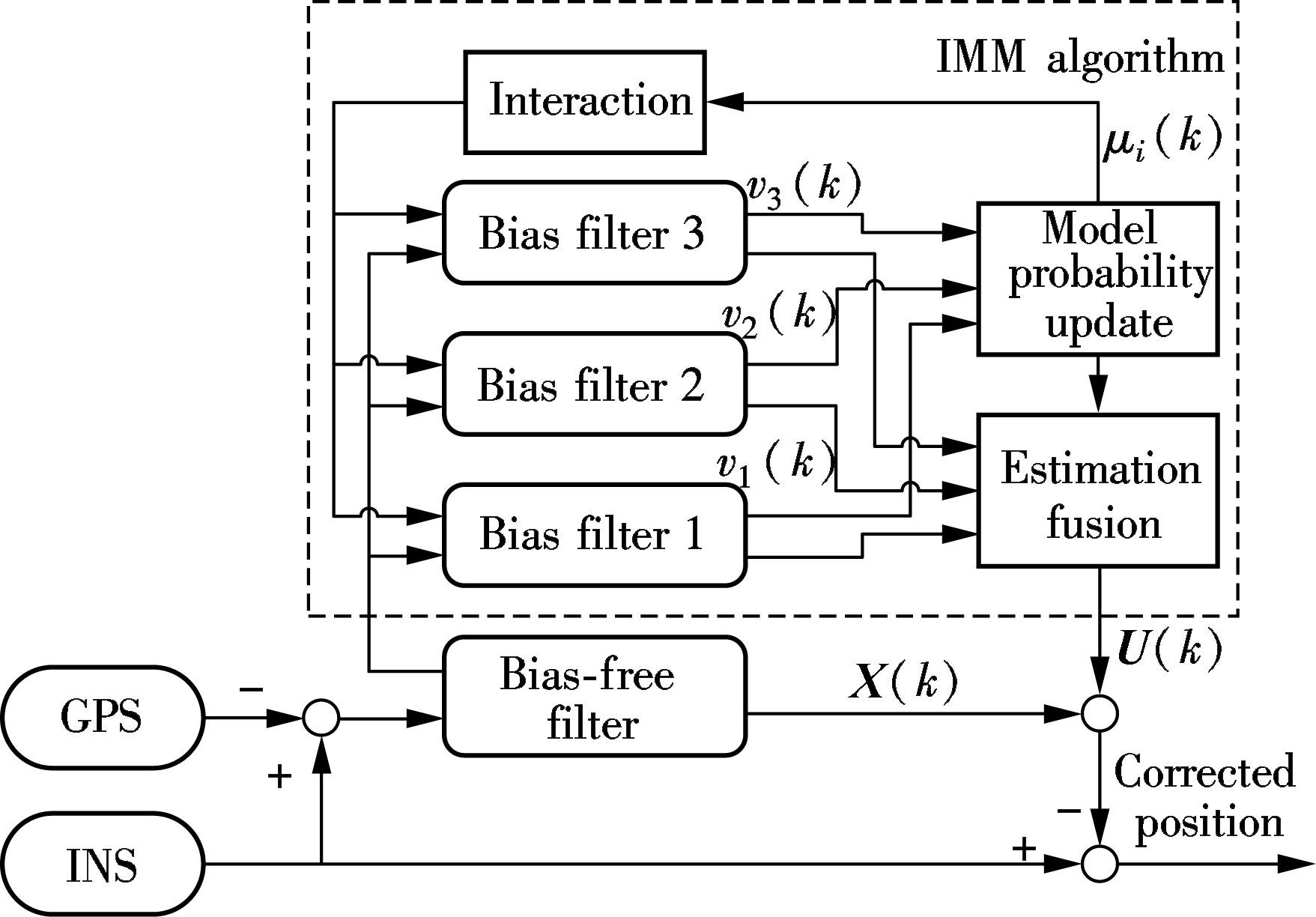
To achieve the target of adapting the uncertain noise of inertial sensors, a novel positioning methodology, termed as IMM-TSKF, is proposed for the INS/GPS integrated positioning system. For further clarification, the whole mechanism and functionality of the proposed positioning methodology is illustrated in Fig.1.
Fig.1 Diagram of the proposed positioning methodology
According to Fig.1, the structure of the two-stage filter is adopted to fuse the information of GPS and INS. The state vector of the bias-free filter is composed of nine navigation parameters, while the accelerometer biases and gyro drifts are included in the state vector of the bias filter. Due to the high uncertainty of MEMS INS noise, the covariances of biases and drifts are difficult to determine. Therefore, three bias filters are developed based on different noise characteristics to cover a large range of noise level, i.e., bias filter 1 for a high noise level, bias filter 2 for normal noise level, and bias filter 3 for low noise level. Finally, the errors of the bias-free filter can be corrected by a weighted sum of the three bias filters, and thereby achieve accurate vehicle positioning. Compared with the conventional two-stage Kalman filter or the augmented state Kalman filter, the proposed methodology is robust to uncertain MEMS INS noise.
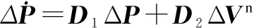
According to INS mechanization, the dynamic error model of the INS navigation parameters (i.e., position, velocity and attitude) can be described as[9]


(1)
where ΔP=[ΔL Δλ Δh]T is the position error vector (latitude, longitude, height); ΔVn=[ΔVE ΔVN ΔVU]T is the velocity error vector (east, north, up); ψn=[ψE ψN ψU]T is the attitude error vector; ![]() is the ideal strapdown matrix;
is the ideal strapdown matrix; ![]() is the angular rate vector of the rotation of the earth relative to the inertial frame;
is the angular rate vector of the rotation of the earth relative to the inertial frame; ![]() is the angular rate vector of the rotation of the navigation frame relative to the earth; fn and Vn are specific force and velocity vectors in the navigation frame, respectively; Δfb and
is the angular rate vector of the rotation of the navigation frame relative to the earth; fn and Vn are specific force and velocity vectors in the navigation frame, respectively; Δfb and ![]() are accelerometer biases and gyroscopes drift vectors in the body frame, respectively; D1 and D2 are two 3×3 matrices, in which the non-zero elements are functions of the vehicle’s latitude and height.
are accelerometer biases and gyroscopes drift vectors in the body frame, respectively; D1 and D2 are two 3×3 matrices, in which the non-zero elements are functions of the vehicle’s latitude and height.
The state vector of the bias-free filter is composed of nine navigation parameter errors (i.e., position error, velocity error, and attitude error), as follows:
X=[ΔL Δλ Δh ΔVE ΔVN ΔVU ψE ψN ψU]
(2)
In this paper, the second-order autoregressive (AR) model is chosen as the error model for accelerometer biases (![]() x,
x, ![]() y,
y, ![]() z) and gyro drifts (εx, εy, εz). The Burg estimation method[10] is applied to determine the parameters of the AR model. The second-order AR model for a discrete-time domain sequence can be described by the following difference equation[11]:
z) and gyro drifts (εx, εy, εz). The Burg estimation method[10] is applied to determine the parameters of the AR model. The second-order AR model for a discrete-time domain sequence can be described by the following difference equation[11]:
y(n)=-α1y(n-1)-α2y(n-2)+β0ω(n)
(3)
where y(n) denotes the observation of the time series; α1 and α2 are the model parameters; and β0 is the standard deviation of the sensor white noise.
It can be seen that for each inertial sensor, the second-order AR model produces two state variables and two coefficients that describe the model. Thus, the state vector of the bias filter can be described as
U= [![]() x1
x1![]() y1
y1![]() z1εx1εy1εz1
z1εx1εy1εz1![]() x2
x2![]() y2
y2![]() z2εx2εy2εz2]T
z2εx2εy2εz2]T
(4)
Based on Eq.(1) and the inertial sensor residual model, the discrete-time system state equation of the two-stage Kalman filter can be presented as[12]
X(k+1)=A(k)X(k)+B(k)U(k)+WX(k)
(5)
U(k+1)=C(k)U(k)+WU(k)
(6)
where A(k), B(k), and C(k) are the state transition matrices; WX(k) is the system noise vector of the bias-free filter with covariance matrix QX(k); and WU(k) is the system noise vector of the bias filter with the covariance matrix QU(k).
The measurement equation can be expressed as
Y(k)=H(k)X(k)+D(k)U(k)+η(k)
(7)
where Y(k) is the measurement vector, which is composed of the differences between the INS measurements and GPS measurements; H(k) and D(k) are the observation matrices; and η(k) is the measurement noise vector with the covariance matrix R.
If the bias and drift term are ignored, the bias-free filter is merely a conventional Kalman filter. Hence, the bias-free filter is given by
X(k,k-1)=A(k-1)X(k-1,k-1)
(8)
PX(k,k-1)=A(k)PX(k,k)A′(k)+QX(k)
(9)
KX(k)= PX(k,k-1)H′(k)·
[H(k)PX(k,k-1)H′(k)+R(k)]-1
(10)
X(k,k)=X(k,k-1)+KX(k)[Y(k)-H(k)X(k,k-1)]
(11)
PX(k,k)=[I-KX(k)H(k)]PX(k,k-1)
(12)
Since the inertial sensor noise is highly uncertain, a fixed value of noise statistics can lead to poor filter performance and even result in filter divergence. Thus, it is advisable to use multiple models, which can represent different noise levels and run in parallel. In our study, the IMM approach contains three bias filters: one for a high noise level, one for normal noise level, and the other for low noise level. The specific IMM approach can be described according to four steps:
Step 1 Interaction
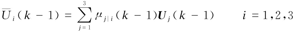
The individual filter estimate Ui(k-1) of the i-th bias filter (i=1,2,3) is mixed with the predicted model probability μi(k-1) and the Markov transition probability πji, i.e. the probability that the transition occurs from state j to state i. The predicted model probability is calculated as
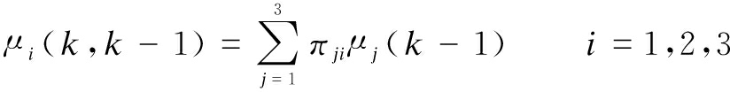
(13)
The mixing weight is given by
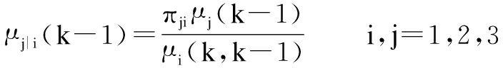
(14)
The mixing state estimation Ui(k-1) is computed as
(15)
The mixing covariance ![]() (k-1) is given as
(k-1) is given as
![]() {
{![]()
![]() } i=1,2,3
} i=1,2,3
(16)
Step 2 Specific filtering
Using the initial mixing state and the covariance of the interacting step, the bias filter with different noise levels predicts and updates the model state and covariance individually. Note that the specification of matrix Q depends on the noise level[13], thus the different bias filter has different matrix Q, i.e. ![]() (i=1,2,3). The execution of the i-th bias filter (i=1,2,3) can be obtained as follows:
(i=1,2,3). The execution of the i-th bias filter (i=1,2,3) can be obtained as follows:

(17)

(18)


(19)

S(k)Ui(k,k-1)]
(20)

(21)
where S(k)=H(k)J(k)+D(k), J(k)=A(k-1)V(k-1)+B(k-1), V(k)=J(k)-KX(k)S(k), and KX(k) is the gain matrix calculated in the bias-free filter.
Step 3 Model probability update
The probability of each model is updated according to the innovation error. Under the assumption of Gaussian statistics, the likelihood for the observation can be calculated from the innovation vector vi(k) and its covariance si(k) is as follows:
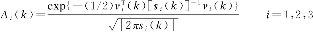
(22)
![]() r.
r.
The model probability update is calculated as
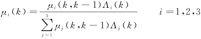
(23)
Step 4 Estimation fusion
The combined state U(k) can be calculated as
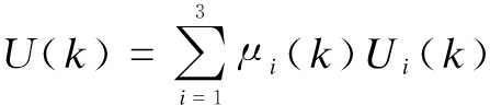
(24)
Then, the estimated U(k) is used to correct the output of bias-free filter X(k) based on Eq.(5). Since the proposed IMM-TSKF methodology can adapt to a wide range of noise levels, an accurate positioning solution can be achieved even when the positioning system suffers from uncertain inertial sensor noise.
The performance of the proposed positioning methodology is examined with several road-test experiments in a land vehicle. Sensor data were collected during the experiments, and the positioning methodologies were run in post-processing using the logged data. The sensor data were recorded via using a Cherry TIGGO 5 SUV vehicle which was equipped with a low-cost NovAtel Superstar Ⅱ GPS receiver with 1 Hz update rate and MEMSIC MEMS-based IMU VG440CA-200 inertial sensors sampled at 100 Hz. For the MEMS-based IMU, each gyroscope has a bias stability of 10 (°)/h and angle random walk of 4.5 (°)/h1/2, while each accelerometer has a bias stability of 1×10⁻³ g and velocity random walk of 1 m/(s·h-1/2). The accuracies of GPS (1σ) are 0.05 m/s for the velocity and 3 m for the position with sufficient satellite signals. Moreover, an accurate and reliable NovAtel SPAN-CPT system was used as a reference for a quantitative comparison. The positioning accuracy of the SPAN-CPT system was 0.01 m with GPS observations.
Several road-test trajectories were carried out using the setup described above. One of the trajectories was carried out in the suburb of Nanjing, China, as shown in Fig.2. This trajectory was in an open field where the number of accessible satellites was greater than five for both the low-cost GPS and SPAN-CPT system throughout the whole procedure of the experiment. Typical driving maneuvers such as turns and stops at the traffic lights were conducted during the test.
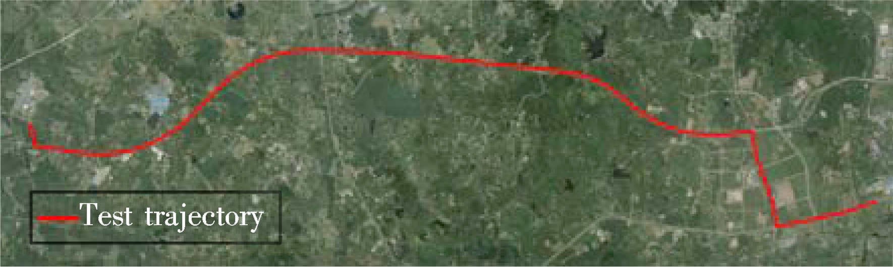
Fig.2 Field test trajectory
The proposed positioning methodology was compared with a general TSKF method. Note that the state vector of the general TSKF is the same as that of IMM-TSKF, i.e. nine elements in the state vector of the bias-free filter and twelve elements in the state vector of the bias filter. However, the general TSKF method has only one bias filter with a constant Q matrix. In addition, the general TSKF method can refer to Ref.[1]. Fig.3 displays the position errors of the integrated positioning system using the two approaches. Note that the position errors denote the horizontal Euclidean distance errors between the estimated position and the corresponding reference.
It can be seen that the proposed IMM-TSKF methodology can achieve better performance than the general TSKF. It can be determined that the average position error of the proposed methodology is 25% lower than that of the general TSKF.
In order to further evaluate the robustness of the IMM-TSKF, we inserted biases in MEMS inertial sensor measurements after 500 s. For convenience and effectiveness, we chose constant biases, i.e. biases of 0.1g into three axes of accelerometers and biases of 300 (°)/h into three
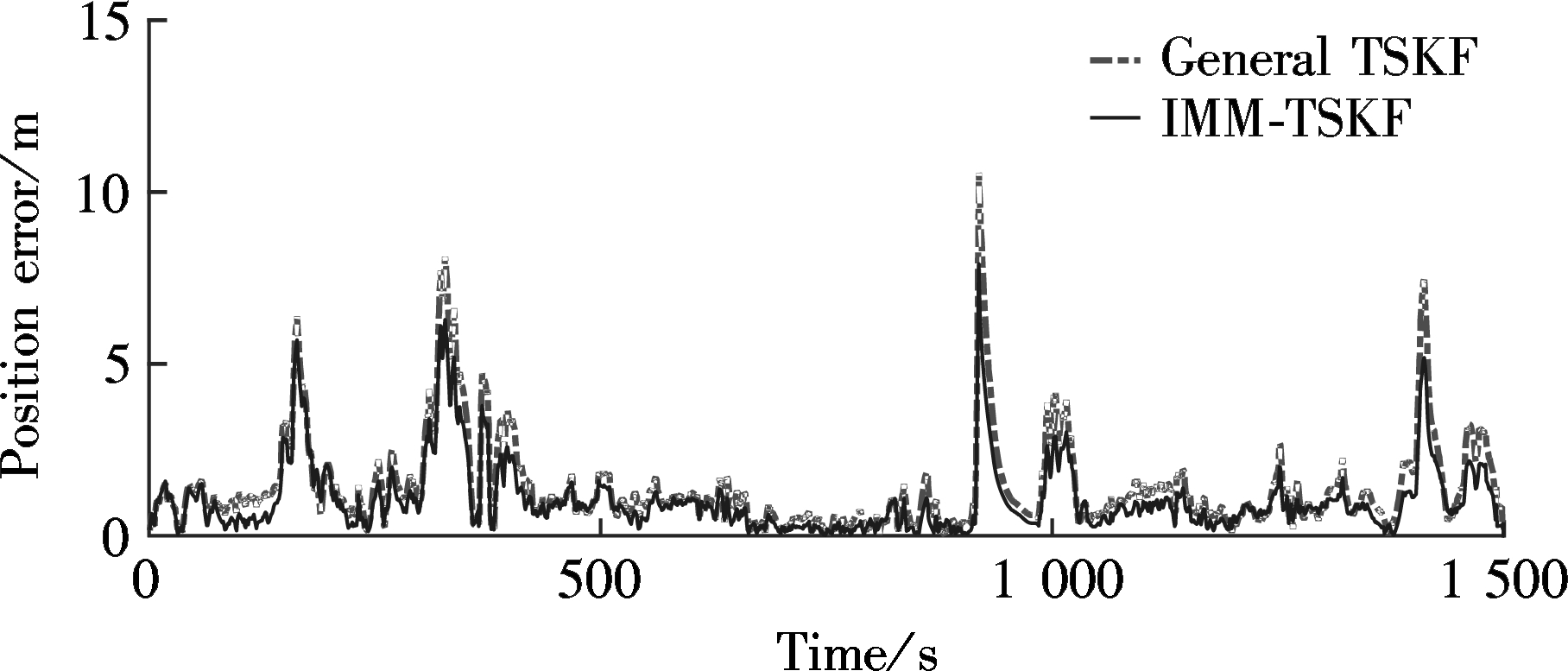
Fig.3 Position errors in general TSKF and IMM-TSKF
axes of gyroscopes. After inserting biases, matrix Q in TSKF needs to be updated correspondingly, which was not done. The inaccurate matrix Q can cause a degradation in TSKF performance. However, IMM-TSKF was envisioned to be adaptive to a wide range of noise levels. Fig.4 shows the results of position errors of the two approaches. It can be seen that the average position error of the proposed methodology is 6.8 m lower than that of the general TSKF after inserting biases.
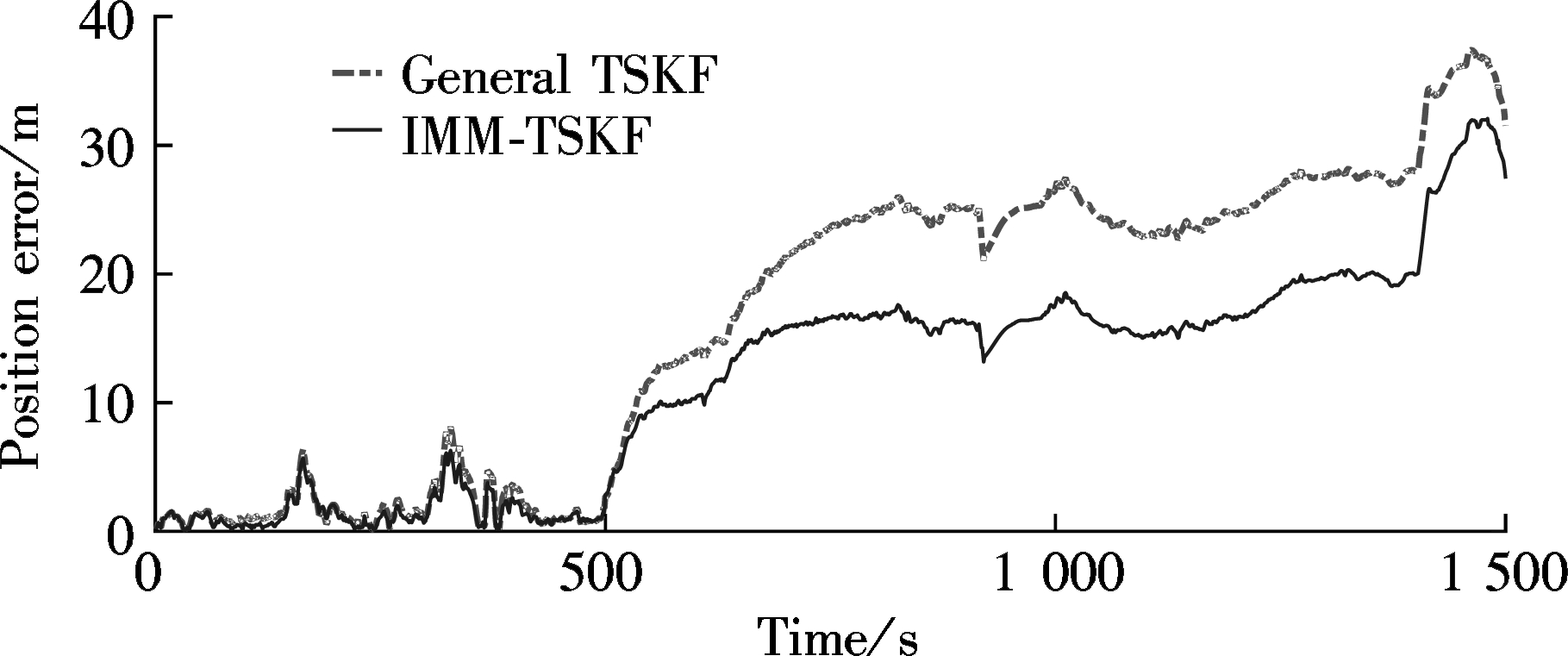
Fig.4 Position errors in general TSKF and IMM-TSKF with inserted biases
This paper proposes a novel positioning methodology for the INS/GPS integration system to adapt to the uncertain noise of MEMS inertial sensors, thereby improving the robustness of the vehicle positioning system. The proposed methodology is based on the structure of the two-stage filter. There are two major advantages: One is that the computational load can be significantly reduced; the other is that it is possible to only adjust the filter involved with accelerometer biases and gyro drifts. Three bias filters are developed to cover a wide range of noise levels. Then, an accurate estimation of biases can be obtained by using the IMM algorithm. Finally, accurate position information can be achieved by removing errors from the output of the bias-free filter. The performance of the proposed methodology is evaluated through typical field tests. The experimental results verify that compared with the general TSKF, the proposed methodology can achieve superior performance.
[1]Kim K H, Lee J G, Park C G. Adaptive two-stage extended Kalman filter for a fault-tolerant INS-GPS loosely coupled system [J]. IEEE Transactions on Aerospace and Electronic Systems, 2009, 45(1):125-137.DOI:10.1109/TAES.2009.4805268.
[2]Feng B, Fu M, Ma H, et al. Kalman filter with recursive covariance estimation—sequentially estimating process noise covariance [J]. IEEE Transactions on Industrial Electronics, 2014, 61(11):6253-6263. DOI:10.1109/tie.2014.2301756.
[3]Ye J, Zhang Z, Shen A, et al. Kalman filter based grid impedance estimating for harmonic order scheduling method of active power filter with output LCL filter [C]//International Symposium on Power Electronics, Electrical Drives, Automation and Motion. Anacapri, Italy, 2016: 359-364.
[4]Lee J Y, Kim H S, Choi K H, et al. Adaptive GPS/INS integration for relative navigation[J]. GPS Solutions, 2016, 20(1): 63-75. DOI:10.1007/s10291-015-0446-4.
[5]Wang Y N, Deng X, Zhao W. Fuzzy Kalman filter based on weighted matrix and its application in integrated navigation [J]. Journal of Chinese Inertial Technology, 2008, 16(3): 334-338.(in Chinese)
[6]Jo K, Chu K, Sunwoo M. Interacting multiple model filter-based sensor fusion of GPS with in-vehicle sensors for real-time vehicle positioning [J]. IEEE Transactions on Intelligent Transportation Systems, 2012, 13(1):329-343. DOI:10.1109/tits.2011.2171033.
[7]Kong J, Zhai X. Application of IMM-Kalman filter algorithm in vehicle navigation system [J]. Computer Engineering and Applications, 2009, 45(14): 198-200. (in Chinese)
[8]Tseng C H, Chang C W, Jwo D J. Fuzzy adaptive interacting multiple model nonlinear filter for integrated navigation sensor fusion [J]. Sensors, 2011, 11(2):2090-2111.DOI:10.3390/s110202090.
[9]Farrell J, Barth M.The global positioning system and inertial navigation [M]. New York: McGraw-Hill, 1999.
[10]Sun Z, Chen Y. Extraction of vortex flowmeter frequency by Burg algorithm based AR model spectral estimation [J]. Journal of Central South University, 2013, 44(4):1684-1688. (in Chinese)
[11]Hao F, Shi J F, Zhang Z S, et al. Image adaptive filtering using general auto-regressive model[J]. Optics & Precision Engineering, 2014, 22(1):186-192.DOI:10.3788/ope.20142201.0186.(in Chinese)
[12]Liu M, Liu Y, Su B K. Application of improved two-stage Kalman filter in error model identification of inertial navigation platform [J]. Journal of Jilin University, 2009, 39(3):819-823. (in Chinese)
[13]Mourikis A I, Roumeliotis S I. A multi-state constraint Kalman filter for vision-aided inertial navigation[C]//2007 IEEE International Conference on Robotics and Automation.Roma, Italy, 2007: 3565-3572.DOI:10.1109/ROBOT.2007.364024.
References:
摘要:为了解决一般状态增强型卡尔曼滤波和两级卡尔曼滤波在微机械惯性传感器不确定噪声的影响下难以获得良好定位性能的问题,提出一种新型的基于交互式多模型的两级卡尔曼滤波方法来适应微机械惯性传感器的不确定噪声.根据不同的噪声特性,建立3个偏差滤波器来覆盖大范围的噪声水平.交互式多模型算法根据3个偏差滤波器可以准确估计出惯性传感器的偏差值,并用来修正无偏差滤波器.因此,应用所提出的滤波方法后,车辆定位系统在不确定噪声的影响下也能获得较好的性能.实验结果显示所提出的交互式多模型两级卡尔曼滤波的平均定位误差比一般两级卡尔曼滤波方法低25%.
关键词:交互式多模型;两级滤波;不确定噪声;车辆定位
中图分类号:U491
Received:2016-09-15.
Foundation item:s:The National Natural Science Foundation of China (No.61273236), the Scientific Research Foundation of Graduate School of Southeast University (No.YBJJ1637),China Scholarship Council.
Citation::Xu Qimin, Li Xu, Li Bin, et al. An interacting multiple model-based two-stage Kalman filter for vehicle positioning[J].Journal of Southeast University (English Edition),2017,33(2):177-181.
DOI:10.3969/j.issn.1003-7985.2017.02.009.
DOI:10.3969/j.issn.1003-7985.2017.02.009
Biographies:Xu Qimin(1989—),male,graduate; Li Xu(corresponding author), male, doctor, associate professor, lixu.mail@163.com.