Abstract:The impact of the adaptive cruise control (ACC) system on improving fuel efficiency is evaluated based on the vehicle-specific power. The intelligent driver model was first modified to simulate the ACC system and it was calibrated by using empirical traffic data. Then, a five-step procedure based on the vehicle-specific power was introduced to calculate fuel efficiency. Five scenarios with different ACC ratios were tested in simulation experiments, and sensitivity analyses of two key ACC factors affecting the perception-reaction time and time headway were also conducted. The simulation results indicate that all the scenarios with ACC vehicles have positive impacts on reducing fuel consumption. Furthermore, from the perspective of fuel efficiency, the extremely small value of the perception-reaction time of the ACC system is not necessary due to the fact that the value of 0.5 and 0.1 s can almost lead to the same reduction in fuel consumption. Finally, the designed time headway of the ACC system is also proposed to be large enough for fuel efficiency, although its small value can increase capacity. The findings of this study provide useful information for connected vehicles and autonomous vehicle manufacturers to improve fuel efficiency on roadways.
Key words:intelligent transportation system; vehicle-specific power; fuel efficiency; energy; connected vehicle; automated vehicle
Fuel consumption and emissions concerns are critical global issues. As the major sector in energy use, the transportation system consumes about 60.3% of oil[1]. Therefore, how to reduce fuel consumption by using innovative technology has become a hot research topic. The adaptive cruise control (ACC) system is the first driver assistance system and mainly focuses on longitudinal behavior, which can maintain a selected velocity and shorter safe time headway by braking and accelerating automatically with a small perception-reaction time. In previous studies, numerous researchers investigated the effects of the ACC system on traffic capacity and safety, and both the positive and negative impacts were proposed[2-6]. Nevertheless, few studies quantified the effect of the ACC system on fuel efficiency. Due to the limitation of the real ACC vehicles on roadways, it is impractical to analyze a large number of ACC vehicles as well as acquire empirical data accordingly. Moreover, the lack of appropriate estimation methods of fuel consumption also restricts the investigation of researchers.
In fact, accurate quantification of fuel use has been a hot research topic in recent years, and numerous estimation models have been proposed at both macroscopic and microscopic levels, such as MOBILE, EMFAC and MOVES[7-8]. Due to the drawback of macroscopic models in their application in transportation projects[7], extensive efforts have been made toward the development of microscopic emission models. Most of the newly developed microscopic models have used the concept of vehicle-specific power VSP[9-10].
The relationship among traffic parameters (speed, grade, acceleration) and fuel efficiency is reflected by VSP. Therefore, it is feasible to use VSP to evaluate the fuel efficiency of ACC vehicles at the microscopic scale. Moreover, as the application of the ACC system is a gradual process, there will be a long period when road traffic consists of ACC and non-ACC vehicles. Different proportions of ACC vehicles will lead to distinct traffic flow features and fuel efficiency impacts, both of which should be particularly investigated. As a fundamental feature of connected vehicles and automated vehicles, the results of this study can also provide useful information for intelligent vehicle design industries to reduce fuel consumption on roadways.
1.1 Development of ACC model
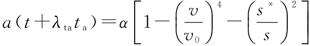
To model ACC vehicles, a method that modifies intelligent driver model (IDM) by augmenting factors is proposed by Kesting et al.[11] and used by numerous researchers. The method is also used in this paper which considered the perception-reaction time factor λta and the safe time headway factor λT. The ACC model derived from the IDM is as follows:
(1)
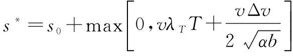
(2)
where ta is the perception-reaction time, s; α is the maximum acceleration, m/s2; v is the speed of the following vehicle, m/s; v0 is the desired speed, m/s; s is the gap distance between two vehicles, m; s0 is the minimum gap distance at standstill, m; T is the safe time headway, s; and b is the desired deceleration, m/s2.
There are several advantages of the proposed ACC model. First, this model was modified from the IDM, which has been proven to be able to model longitudinal driving behavior accurately. Therefore, the developed ACC model can conform to people’s driving habits to some degree. Moreover, the ACC model not only considers drivers’ behavior but represents the essential features of this advanced driving-assistant system, the perception-reaction time factor λta and the safe time headway factor λT. Note that the two factors, the maximum acceleration a and the desired deceleration b, proposed by Kesting et al.[11] are not modified. The reason is that the authors believe these two parameters are limited by the engine power of vehicles and the comfort of humans, which cannot essentially be improved by the ACC systems. Finally, another advantage is that the calibration of the proposed model is simple. Although large scale experiments on a production ACC vehicle are not practical, the ACC model can be calibrated indirectly by determining the values of parameters in the basic IDM with empirical data and by adjusting the crucial factors λta and λT accordingly. It is a reasonable alternative considering the lack of data on a large number of real ACC vehicles.
1.2 Model calibration
In order to use the fuel efficiency indicator developed by Song and Yu[12] precisely, the IDM was first calibrated using empirical data. The urban traffic data of the same type of gasoline-fueled light-duty vehicle was collected on Beijing Xi road in Nanjing during the peak hour from October 19 to October 23, 2009. 20 drivers participated in the experiment and the vehicle was equipped with a high-precision GPS receiver and a digital laser rangefinder collected a total of 6 306 records of trajectory data. All the trajectories longer than 15 s were selected as proper data. These trajectory data include the position, the speed and the acceleration of each vehicle at each second. The basic IDM is calibrated with the second-by-second traffic data by minimizing the difference between the discrete traffic data of observation and model estimation. The minimization objective function includes both the observed spacing headway and model estimated spacing headway, which is defined as[13]

(3)
β*=argminεmodel(β)
(4)
where ![]() is the spacing headway of the observation;
is the spacing headway of the observation; ![]() is the spacing headway of the model estimation; β is the parameter vector needing calibrated; i is the sequence number of sample points; j is the sequence number of trajectory; nj is the total number of sample points in the j-th trajectory; J is the number of trajectories used in the model calibration for a certain participant; and β* is the calibrated parameter vector.
is the spacing headway of the model estimation; β is the parameter vector needing calibrated; i is the sequence number of sample points; j is the sequence number of trajectory; nj is the total number of sample points in the j-th trajectory; J is the number of trajectories used in the model calibration for a certain participant; and β* is the calibrated parameter vector.
By minimizing the calibration error, the best parameter value of the IDM is found, as shown in Tab.1.
Tab.1 Calibrated values of parameters in the IDM
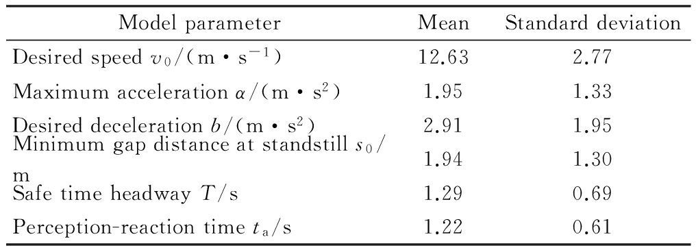
ModelparameterMeanStandarddeviationDesiredspeedv0/(m·s-1)12.632.77Maximumaccelerationα/(m·s2)1.951.33Desireddecelerationb/(m·s2)2.911.95Minimumgapdistanceatstandstills0/m1.941.30SafetimeheadwayT/s1.290.69Perception-reactiontimeta/s1.220.61
On the basis of the calibration values of the basic IDM with empirical data, the ACC model can be determined by setting the values of λta and λT. In this paper, the two values λtata and λTT are initially set to be 0.1 and 0.9 s, respectively. The former value of 0.1 s of modified perception-reaction time is assumed to be the technical minimum of ACC vehicles, and the latter one is set according to the previous study of Kesting et al.[14], in which λT equals 0.7. Furthermore, considering that the two factors are crucial to the performance of ACC vehicles, the sensitivity analyses of these factors are also conducted in simulation experiments to investigate the impacts of different factor values on fuel efficiency.
2.1 Fuel efficiency indicator
VSP is a proxy variable of engine load, W/kg. For a typical light-duty vehicle, VSP can be calculated as
VSP=v(1.1a+9.81g+0.132)+0.000 302v3
(5)
where v is the speed of vehicles, m/s; a is the acceleration of vehicles, m/s2; and g is the vehicle vertical rise divided by slope length,%.
A method that develops the relationships between second-by-second speed and acceleration data with fuel efficiency was proposed by Song and Yu[12] based on VSP, which performs well in evaluating fuel efficiency in road traffic. For the detailed process, one can refer to the paper of Song and Yu[12,15-16]. In this study, this process is simply introduced in the following five steps:
Step 1 Calculate VSP using second-by-second speed and acceleration data. For a typical light-duty vehicle simulated in this paper, in which g is assumed to be 0, the value of VSP can be calculated as
VSP=v(1.1a+0.132)+0.000 302v3
(6)
Step 2 Calculate VSPbin for each VSP value in Step 1. VSPbin is applied by numerous studies[12,15-16] to avoid random errors resulting from second-by-second data. VSPbin is calculated as
VSPbin=n ∀VSP∈[n-0.5, n+0.5)
(7)
where n is the number of VSPbin.
Step 3 Estimate the normalized fuel consumption rate NFR for each VSPbin. NFR was proposed by Song and Yu[12] in which the average fuel consumption rates are divided by the idling rate to eliminate the impacts of different engine size, fuel type, and vehicle mass on absolute fuel consumption rates. According to Song’s study[12], 26 sampled light-duty vehicles consistently show that each VSPbin matches a fixed NFR equal to 1 in negative values, and can be expressed by using the same power function of VSP in the positive values. Song and Yu[12] believed that the consistency of NFR may be attributed to the similarities in vehicles and technologies. Therefore, in this paper, the same type light-duty vehicle is used to collect traffic data on the similar urban roadway. The regression equation of NFR with VSP in the positive part developed in Ref.[12] is also applied in this paper, which is expressed as
NFR=1.71(VSPbin)0.42
(8)
The average NFR can be calculated as

(9)
where i is the number of VSPbin; NAFR is the average NFR; Ti is the time fraction.
Step 4 Calculate the average normalized fuel factor NFF. The average NFR for road traffic reflects the fuel consumption per unit of time. However, in real networks, the factor NAFF, indicating the fuel consumption per unit of distance is more practical and valuable. Therefore, the average NFF introduced by Song and Yu[12] is expressed as
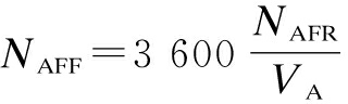
(10)
where NAFF is the average NFF; VA is the average travel speed.
Step 5 Calculate the fuel efficiency indicator FEI for road traffic and FEI is defined as
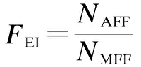
(11)
where NMFF is the special constant calculated based on the assumption that vehicles travel at the most efficient speed. The speed reflects the normalized fuel consumption per unit of distance in the most economic scenario, and it is equal to 162.5 according to Ref.[12]. By using the above five-step process, a relationship can be established between second-by-second data of each vehicle and the fuel efficiency indicator.
2.2 Design of simulation experiment
The experiments of this research were based on the simulation platform coded in Matlab software. The basic IDM and ACC model calibrated in the above section were used to model non-ACC and ACC vehicles, respectively. Note that lane-changing behavior was not included in simulations due to the deficiency of proper models for lane-changing in existing literature. Moreover, speed reductions related to fuel consumption on urban roads are mainly caused by car-following behavior instead of lane-changing. Then FEI was calculated based on the five-step process to evaluate the impacts of ACC systems on fuel efficiency. Five scenarios were tested with various proportions of ACC vehicles including 0%-ACC, 10%-ACC, 30%-ACC, 50%-ACC, and 100%-ACC.
The major section of Beijing Xi road was used to simulate the roadway section. The 3.1-km roadway section with three lanes in one direction was considered in simulation experiments. Four intersections were simplified as the factor to brake and accelerate vehicles, which led to the speed variation of vehicles and fluctuation of traffic flow. Moreover, the fluctuation can significantly show the difference between ACC and non-ACC vehicles. Each simulation lasted 0.5 h with a time step of 1 s. The first five minutes were considered the warm-up period and the traffic demand was set to be 800 pcu/(h·lane-1). For each scenario, the second-by-second discrete speed and acceleration data of each vehicles were generated and FEI was calculated by using the five-step process. The values of FEI were compared and discussed in the following section and the sensitivity analyses were also conducted.
3.1 Impacts of ACC on fuel efficiency
FEI indicates the average fuel efficiency of all the vehicles on a roadway or a network, and the smaller the value, the more efficient the fuel consumption. The simulation results of five scenarios are illustrated in Fig.1.
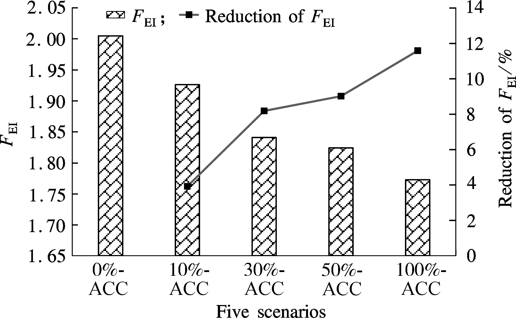
Fig.1 FEI results of five different scenarios
In general, compared with the 0%-ACC scenario, all the other four scenarios with different ACC proportions have smaller FEI values. The result is in accordance with previous study and is reasonable due to ACC vehicles smooth traffic flow by accelerating and braking automatically with a shorter time delay. The avoidance of abrupt acceleration and deceleration reduces the fuel consumption effectively. Furthermore, the ACC system has a smaller FEI with the increasing penetration rate of ACC. For example, the scenario with 10%-ACC only reduces FEI by 3.92% compared with 0%-ACC, which indicates that the small proportion of ACC in traffic can slightly improve the traffic operation and fuel consumption. For the 100%-ACC scenario, however, the FEI value is reduced by 11.58%. Note that the reduction of 11.58% is significant when fuel consumption of all the vehicles in the network are summarized based on FEI. With all the vehicles on the roadway equipped with ACC systems, the traffic operation will be improved significantly, and the redundant fuel consumption of abrupt deceleration can be reduced effectively. The FEI of 30%-ACC and 50%-ACC scenarios are also reduced by 8.18% and 9.01%, respectively. This result is interesting since only 30% ACC vehicles can also have relatively greater fuel consumption benefits compared with 100%-ACC. In the future market, it is difficult for all the vehicles to equip themselves with ACC systems in a short term. However, keeping the market penetration rate of ACC to 30% is feasible and effective, considering the relatively large reduction in fuel consumption.
3.2 Sensitivity analysis of λta and λT
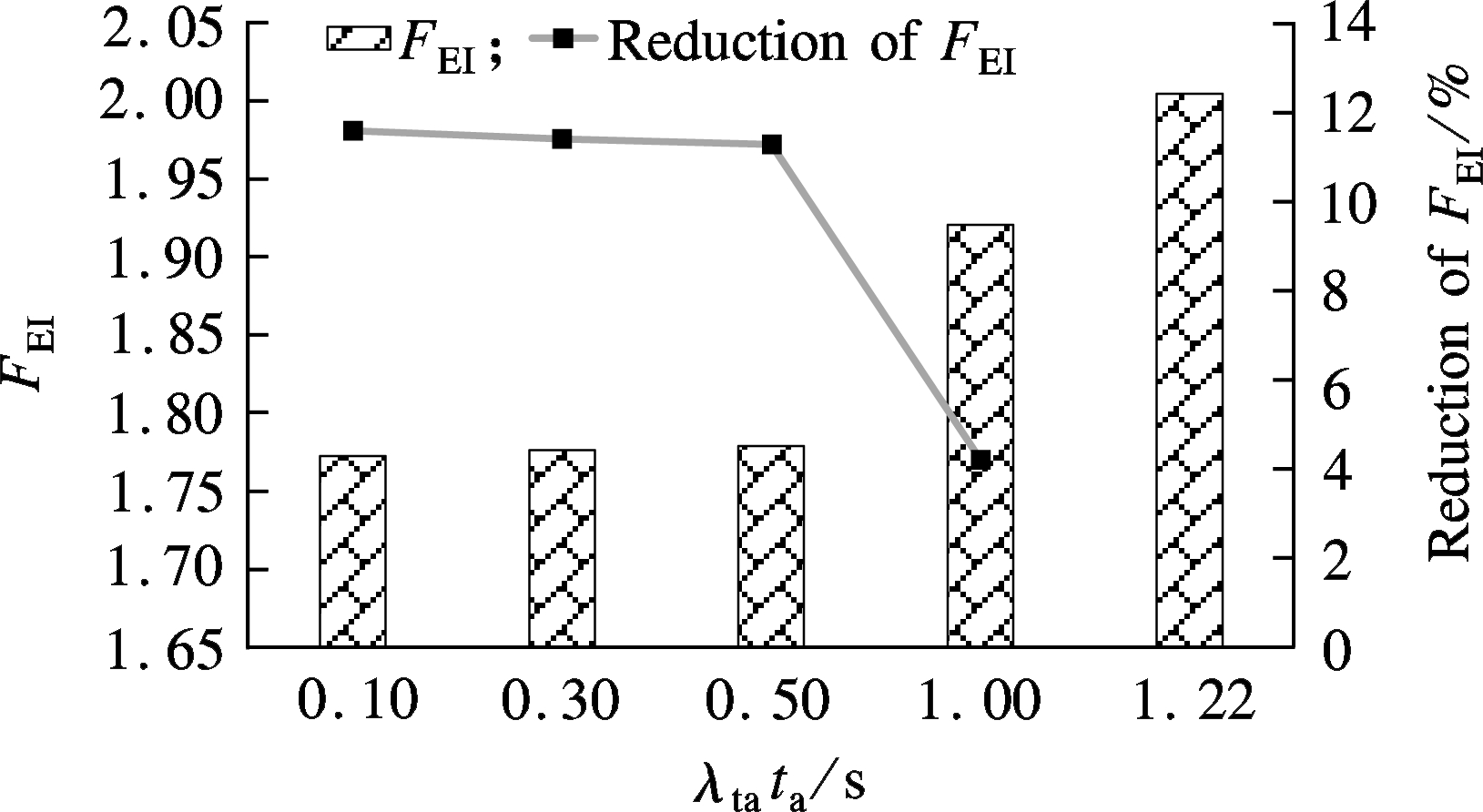
As shown in Fig.2(a) and Tab.2, 100%-ACC scenario with four different values of λtata are tested in simulations compared with 0%-ACC scenario. It is clear that the ACC vehicles with shorter perception-reaction time have smaller FEI values. The shorter time delays of vehicles can reduce the variation of velocities and acceleration, which consequently leads to fuel consumption advantages. The FEI value is reduced by only 4.19% with λtata of 1 s. The difference of perception-reaction time is small compared with the 0%-ACC vehicles of 1.22 s. However, ACC vehicles with λtata of 0.5 s can reduce the FEI value significantly by 11.27%. The FEI values of ACC vehicles with smaller λtata decrease slightly compared to scenarios with a perception-reaction time of 0.5 s. As shown in Tab.2, scenarios with λtata of 0.1 and 0.3 s can reduce FEI by 11.58% and 11.40%, respectively. The result provides useful information for vehicle industries stating that the perception-reaction time of the ACC system only needs to be of a relatively small value to obtain relatively greater fuel consumption benefits.
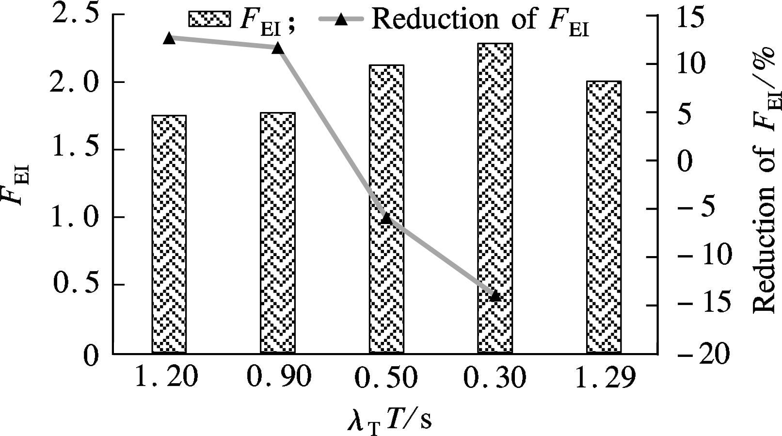
A sensitivity analysis of λT is also conducted and shown in Fig.2(b) and Tab.2. 100%-ACC scenariowith different λTT values are investigated The results of the non-ACC scenario is used as the basic line for comparison. The FEI of non-ACC scenario is 2. The smaller λTT value represents the shorter time headway of ACC, which can lead to larger capacity according to some research. However, it is obvious that a shorter time headway of the leading and following vehicles can easily result in rear-end collision and the abrupt deceleration of the following vehicle, which is not beneficial for fuel consumption saving. The results are in line with the above analysis. ACC vehicles with a large time headway of 0.9 and 1.2 s can reduce the FEI values by 12.59% and 11.58%, respectively. For the scenarios with time λTT of 0.5 and 0.3 s, the FEI values are increased by 6.04% and 14.08%, respectively. The result is crucial since the time headway of the ACC system cannot be set to be very small to increase capacity. The relatively large headway is required from the perspective of fuel efficiency.
(a)
(b)
Fig.2 FEI results with different parameters. (a) Perception-reaction time; (b) Time headway
Tab.2 FEI values of different perception-reaction time and time headway

Itemλtata0.1s0.3s0.5s1sλTT1.2s0.9s0.5s0.3sFEI1.771.781.781.921.751.772.132.29ReductionofFEI/%-11.58-11.40-11.27-4.19-12.59-11.586.0414.08
In the above simulation, there were four intersections in the urban road. The number of intersections, however, also has impacts on the result. Thus, another four scenarios were considered, which assumed that there are three, two, one and no intersections in simulations. The perception-reaction time and time headway were set to be 0.1 and 0.9 s. The sensitive analysis result of different numbers of intersections are illustrated in Tab.3. The non-ACC scenario is also used as the basic line for comparison. With the increase of the intersection number, the reduction of FEI decreases apparently, from 21.86% to 11.58%. This result is intuitively rational since ACC vehicles decelerate more frequently when approaching more intersections. This result also indicates that the green wave design, which reduces the intersection number equally, may be beneficial for fuel efficiency improvement.
Tab.3 Reduction of different numbers of intersections

ItemNumberofintersections01234ReductionofFEI/%-21.86-19.70-15.81-13.54-11.58
This study evaluates the fuel efficiency of ACC vehicles on a roadway based on VSP. First, the IDM was modified to simulate ACC behaviors, and it was also calibrated by using empirical trajectory data. Then, FEI was calculated by the five-step process. Five scenarios, i.e., 0%-ACC, 10%-ACC, 30%-ACC, 50%-ACC and 100%-ACC, were considered in the simulation experiments. Furthermore, sensitivity analyses were also conducted to investigate the impact of different values of the two key factors affecting perception time and time headway. The results show that, compared to the 0%-ACC scenario, all the scenarios with different penetration rates of ACC vehicles have a positive effect on reducing fuel consumption. The FEI value of 10%-ACC is reduced by 3.92%, while the values of 30%-ACC and 100%-ACC scenarios are reduced by 8.18% and 11.58%, respectively. The sensitivity analyses of λta and λT show that a smaller perception-reaction time of ACC vehicles has better fuel efficiency benefits, while on the contrary, a shorter time headway can increase the fuel consumption.
[1]International Energy Agency. Key world energy statistics [R]. Paris: International Energy Agency, 2007.
[2]Li Y, Wang H, Wang W, et al. Reducing the risk of rear-end collisions with infrastructure-to-vehicle (I2V) integration of variable speed limit control and adaptive cruise control system [J]. Traffic Injury Prevention, 2016, 17(6): 597-603. DOI:10.1080/15389588.2015.1121384.
[3]Tapani A. Vehicle trajectory effects of adaptive cruise control [J]. Journal of Intelligent Transportation Systems, 2012, 16(1): 36-44. DOI:10.1080/15472450.2012.639641.
[4]Li Y, Wang H, Wang W, et al. Evaluation of the impacts of cooperative adaptive cruise control on reducing rear-end collision risks on freeways [J]. Accident Analysis and Prevention, 2017, 98: 87-95. DOI:10.1016/j.aap.2016.09.015.
[5]Carbaugh J, Godbole D N, Sengupta R. Safety and capacity analysis of automated and manual highway systems [J]. Transportation Research Part C: Emerging Technologies, 1998, 6(1): 69-99. DOI:10.1016/s0968-090x(98)00009-6.
[6]Chira-Chavala T, Yoo S M. Potential safety benefits of intelligent cruise control systems [J]. Accident Analysis and Prevention, 1994, 26(2): 135-146. DOI:10.1016/0001-4575(94)90083-3.
[7]Barth M, An F, Younglove T, et al. Comprehensive modal emission model (CMEM) [M]. 2nd ed. Riverside: University of California Press, 2000.
[8]Vallamsundar S, Lin J. MOVES versus MOBILE: Comparison of greenhouse gas and criterion pollutant emissions [J]. Transportation Research Record: Journal of the Transportation Research Board, 2011, 2233: 27-35. DOI: 10.3141/2233-04.
[9]Davis N, Lents J, Osses M, et al. Part 3: Developing countries: Development and application of an international vehicle emissions model [J]. Transportation Research Record: Journal of the Transportation Research Board, 2005, 1939: 155-165. DOI:10.3141/1939-18.
[10]United States Environmental Protection Agency. Draft motor vehicle emission simulator (MOVES) user guide [R]. Washington DC: USEPA, 2009.
[11]Kesting A, Treiber M, Schönhof M, et al. Jam-avoiding adaptive cruise control (ACC) and its impact on traffic dynamics [M]//Traffic and Granular Flow’05. Heidelberg: Springer, 2007: 633-643.
[12]Song G H, Yu L. Estimation of fuel efficiency of road traffic by characterization of vehicle-specific power and speed based on floating car data [J]. Transportation Research Record: Journal of the Transportation Research Board, 2009, 2139: 11-20. DOI:10.3141/2139-02.
[13]Wang H, Wang W, Chen J, et al. Using trajectory data to analyze intradriver heterogeneity in car-following [J]. Transportation Research Record: Journal of the Transportation Research Board, 2010, 2188: 85-95. DOI:10.3141/2188-10.
[14]Kesting A, Treiber M, Helbing D. Enhanced intelligent driver model to access the impact of driving strategies on traffic capacity [J]. Philosophical Transactions of the Royal Society of London A: Mathematical, Physical and Engineering Sciences, 2010, 368(1928): 4585-4605. DOI:10.1098/rsta.2010.0084.
[15]Song G H, Yu L, Zhang Y H. Applicability of traffic microsimulation models in vehicle emissions estimates: Case study of VISSIM [J]. Transportation Research Record: Journal of the Transportation Research Board, 2012, 2270: 132-141. DOI:10.3141/2270-16.
[16]Song G H, Yu L, Xu L. Comparative analysis of car-following models for emissions estimation [J]. Transportation Research Record: Journal of the Transportation Research Board, 2013, 2341: 12-22. DOI:10.3141/2341-02.
References:
摘要:基于车辆比功率评价了自动巡航控制系统对改善油耗效率的影响.首先改进了智能驾驶员模型来模拟自动巡航控制系统,并用实测交通数据进行了标定;然后基于车辆比功率提出了一个五步过程用于计算油耗效率.通过仿真实验测试了不同比例自动巡航控制系统下的5种方案,同时对影响自动巡航控制系统感知反应时间和车头时距的2个关键因素进行了敏感性分析.仿真结果表明,所有采用自动巡航控制车辆的方案对减少油耗有积极影响,此外,从油耗效率的角度来看,并不需要采用很小的感知反应时间值,因为该值取0.5 ~ 0.1 s几乎带来相同的油耗减少效果.最后,虽然较小的车头时距可以提高通行能力,但就油耗效率而言该值需要设计得足够大.研究结果可为连接车和自动车辆设计行业改善道路油耗效率提供有效信息.
关键词:自动巡航控制;车辆比功率;油耗效率;能源;连接车;自动车
中图分类号:U491
Received:2016-12-16.
Foundation item:The National Natural Science Foundation of China (No.51338003, 51478113, 51378120).
Citation::Li Ye, Wang Wei, Wang Hao, et al. Evaluation of the impacts of adaptive cruise control system on improving fuel efficiency of urban road traffic[J].Journal of Southeast University (English Edition),2017,33(2):230-235.
DOI:10.3969/j.issn.1003-7985.2017.02.017.
DOI:10.3969/j.issn.1003-7985.2017.02.017
Biographies:Li Ye (1992—),male,graduate; Wang Wei (corresponding author), male, doctor, professor, wangwei@seu.edu.cn.