Abstract:The flexibility of dynamic community structure is adopted to analyze the depressive resting-state functional magnetic resonance imaging (rfMRI) signals in order to improve the accuracy of evaluating depression treatment. The rfMRI signals of each brain network were obtained by the independent component correlation algorithm (ICA). Dynamic functional connections were computed with sliding windows and L1 norm. Then, the connections were used to calculate the dynamic community structure via the community-detection algorithm. The result of structure’s community assignment has the general character with the brain activity changing over time. The flexibility index is one of traits of dynamic community structure, meaning the number of times a region changes. In this study, 16 patients who achieved clinical remission joined the experiment and were scanned before and after treatment. Pair permutation tests compare the difference of six brain networks’ flexibility between pre-therapy and post-treatment. The results show that the distribution of the flexibility values declines in a default network and cognitive control network between pre-therapy and post-treatment patients with statistical difference. Therefore, flexibility is a suitable approach to accurately evaluate the depression treatment effect.
Keywords:dynamic community structure; magnetic resonance imaging (MRI); depression; treatment effect
Resting-state functional magnetic resonance imaging (rfMRI) was not regarded as a temporal stationarity and the sliding time window was used to calculate the dynamic functional connectivity (FC) and study the temporal variability of brain activity[1]. The dynamic FCs were obtained by the way of spatial independent component analysis or region of interest (ROI), and then they were clustered into suitable groups to investigate brain dynamics[2]. However, this type of method ignored the coupling relations of adjacent layers of the sliding time window and cannot express the time-dependence during the brain activity.
Dynamic community structure removes above limits via quality functions to multislice networks and dynamic network null models were found to certify the robustness of the dynamic community structure[1]. This algorithm of studying dynamic brain activity has been used to study the dynamic reconfiguration of human brain networks during learning and different dynamic brain activities between depression and matched health[2-4].
Flexibility is one of dynamic community structure’s traits, which means the normalized number of times a region changes and manifests the dynamic activity of a node[3]. The network flexibility increases and then decreases during a learning process and network flexibility values were modulated by learning[3]. The flexibility of the salience network was significantly different between depression and health[4]in our previous work. Therefore, it is necessary to explore further whether such a network characteristic can identify the status of patients pre/post treatment.
In this article, dynamics community structure was used to compute the whole brain’s region community assignment with time and flexibility is the model’s trait to distinguish between the pre-therapy and post-treatment. The method of spatial independent component analysis (ICA) together with the sliding time windows is used to extract the resting state network signals and then to compute the dynamic FC. Then dynamics community structure and flexibility can be calculated via dynamic FC to detect the transformation of dynamic brain activity.
1.1 Community detection algorithm
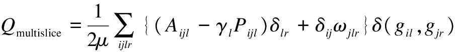
Dynamic community structure is composed by community-detection algorithms. The community-detection algorithm divides a network into several connected tightly groups of nodes[1]. The connected dense of nodes in a group is above the level between nodes in different groups. We established coupling relationships between layers by sliding windows. In this algorithm,Aijlgives the connection of layer-landPijloffers the constituent of the relevant layer-lconnection for the optimization null model. The maximum value ofQis a key index when dividing the network into groups. For example, the total connection weight inside the group is allowed to be as large as possible. Then, the algorithm can be defined as[5]
whereδijωijlis the coupling relationship between layers andωjlrmeans the coupling connection strength. The Kronecker deltaδij=1 ifi=jandδij=0 otherwise.γlis layerl’s structural resolution parameter andgilrepresents the community assignment in nodeiand layerl. Meanwhile, the sum of the whole network’s edge weight givesμ=![]() Kjrand the power in nodejand layerlequalsKjl=kjl+cjlwhen the strength of inter-layer and intra-layer in nodejin layerlis calculated viakjl=
Kjrand the power in nodejand layerlequalsKjl=kjl+cjlwhen the strength of inter-layer and intra-layer in nodejin layerlis calculated viakjl=![]() Aijlandcjl=
Aijlandcjl=![]() ωjir.
ωjir.
1.2 Dynamic network null models
Dynamic network null models consist of a connectional null model, a nodal null model, a temporal null model and the result’s robustness in changing intra-layer strength between layers[2,5]. A connectional null model, a nodal null model and a temporal null model are the permuted networks for the connectional, nodal, and temporal null models, respectively[2].
2.1 Participants
All participants were patients with a depressive episode who were from 20 to 55 years of age. 30 participants were selected to join the experiment but only 16 achieved clinical remission after treatment which was confirmed by expert psychiatrists and conducted the whole experiment.
The 16 participants consist of 12 males and 4 females. The mean of patients’ age and education years are 37.125 and 12.938, respectively. The average value and standard deviation of patients’ HDRS (Hamilton depression rating scale) are 25.500 and 5.562 before treatment and are 4.875 and 4.515 after treatment. Thepvalue of the two-tailed t-test is significantly different between pre-therapy’s HDRS and post-treatment’s HDRS.
The initial diagnoses of depressive episode patients were made by patients’ treating psychiatrists and confirmed by an expert psychiatrist according to the Diagnostic and Statistical Manual of Mental Disorders 4th (DSM-Ⅳ) criteria. They were assessed using 17-item Hamilton Rating Scale for Depression at the first scans and second scans.
2.2 Image data acquisition
All patients were scanned by the 3.0-T Siemens MRI system (Siemens Medical Solutions, Germany). All T1-weighted structural data and the resting-state functional images were recorded by a gradient-echo sequence with the following scanning parameters as summarized in Tab.1. Every functional image scan obtained 133 volumes and all participants kept the eyes closed and thought of nothing during scanning time.
2.3 Data preprocessing
The first five functional volumes were deleted to let participants adapt to the machine noise. Data preprocessing was handled via DPARSF and the steps include slice-timing, head-motion correction, normalization, and smoothing[6]. Structural data was allowed to segment and transform into the Montreal Neurological Institute (MNI) space and its resolution parameter is 3 mm×3 mm×3 mm. Then, smoothing was done to the functional image with 6-mm full-width at half-maximum Gaussian kernel.
Tab.1 The major parameters of image data acquisition
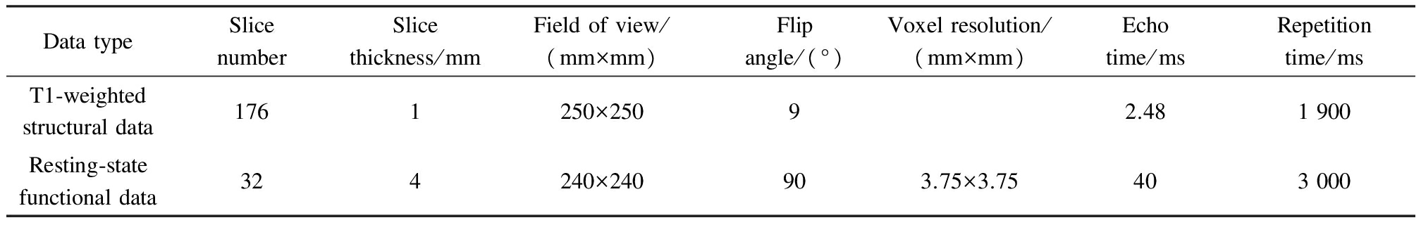
DatatypeSlicenumberSlicethickness/mmFieldofview/(mm×mm)Flipangle/(°)Voxelresolution/(mm×mm)Echotime/msRepetitiontime/msT1⁃weightedstructuraldata1761250×25092.481900Resting⁃statefunctionaldata324240×240903.75×3.75403000
2.4 Group spatial independent component correlation algorithm
Group spatial ICA (independent component correlation algorithm) was used on every group’s data, respectively, by GIFT software[7]. Images were imported into the toolbox and rfMRI signals were divided into one hundred groups of independent components when the informax algorithm was repeated 10 times to guarantee the robustness of the Group spatial ICA[8]. Individuals’ time courses in these spatial independent components were then estimated by the GICA3 back-reconstruction algorithm. Independent components of six networks in the whole brain were selected by visual identity and correlation templates mapping with Allen’s result[9]. Groups of pre-therapy, post-treatment were handled, respectively, and the number of independent components was a little different in the two groups. The results after Group spatial ICA were bandpass filtered (0.01 to 0.08 Hz) to reduce low-frequency drift and high-frequency noise before calculating covariance.
2.5 Dynamic functional connection estimation
Every covariance of sliding windows was calculated. We used a rectangular window with steps of 3 s. The width of a rectangular window is 90 s and the number of windows is 99. At the same time, the L1-norm regularized precision matrix was used to estimate every window’s covariance due to the stability of short time window segments and keep the sparseness of precision matrix[8]. Then, individual’s dynamic functional connections were estimated by the precision matrix[9-10].
2.6 Dynamic community structure
According to relevant papers, the structural resolution parameter and the intra-layer connection between layers were both set to be 1.0 in this experiment[9]. A participant’s dynamic community structure was calculated 100 times and the mean ofQvalues was taken as the final result due to the local optimum of the algorithm. However, for all participants, the result of the algorithm is convergent and the discrepancy of everyQvalue was extremely small between 100 times’ computation[3,7]. Fig.1 gives one participant’s distribution ofQafter 100 times computation. Fig.2 gives a dynamic community structure’s community assignment and the dynamic interaction between nodes during the scanning.
The results of the pair permutation test show that the distribution of theQvalues and module number are non-significant between two groups. However, the distributionsof index called flexibility were significantly different in the default networks and cognitive control networks between pre-therapy and post-treatment (see Tab.2).
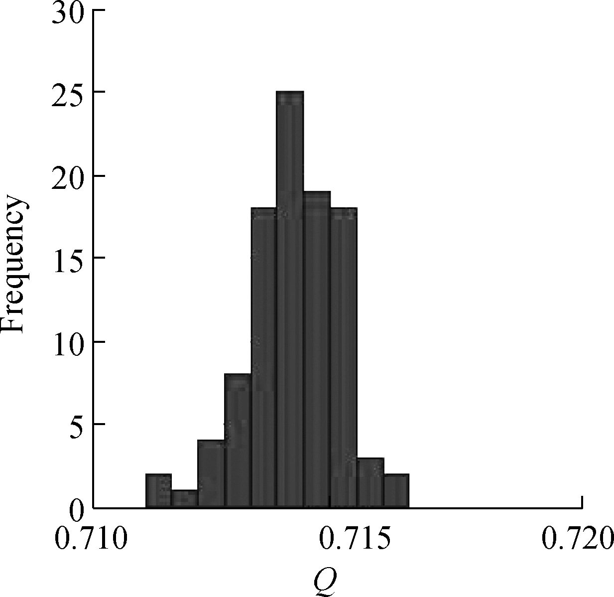
Fig.1 A participant’s distribution ofQbetween 100 times’ computation
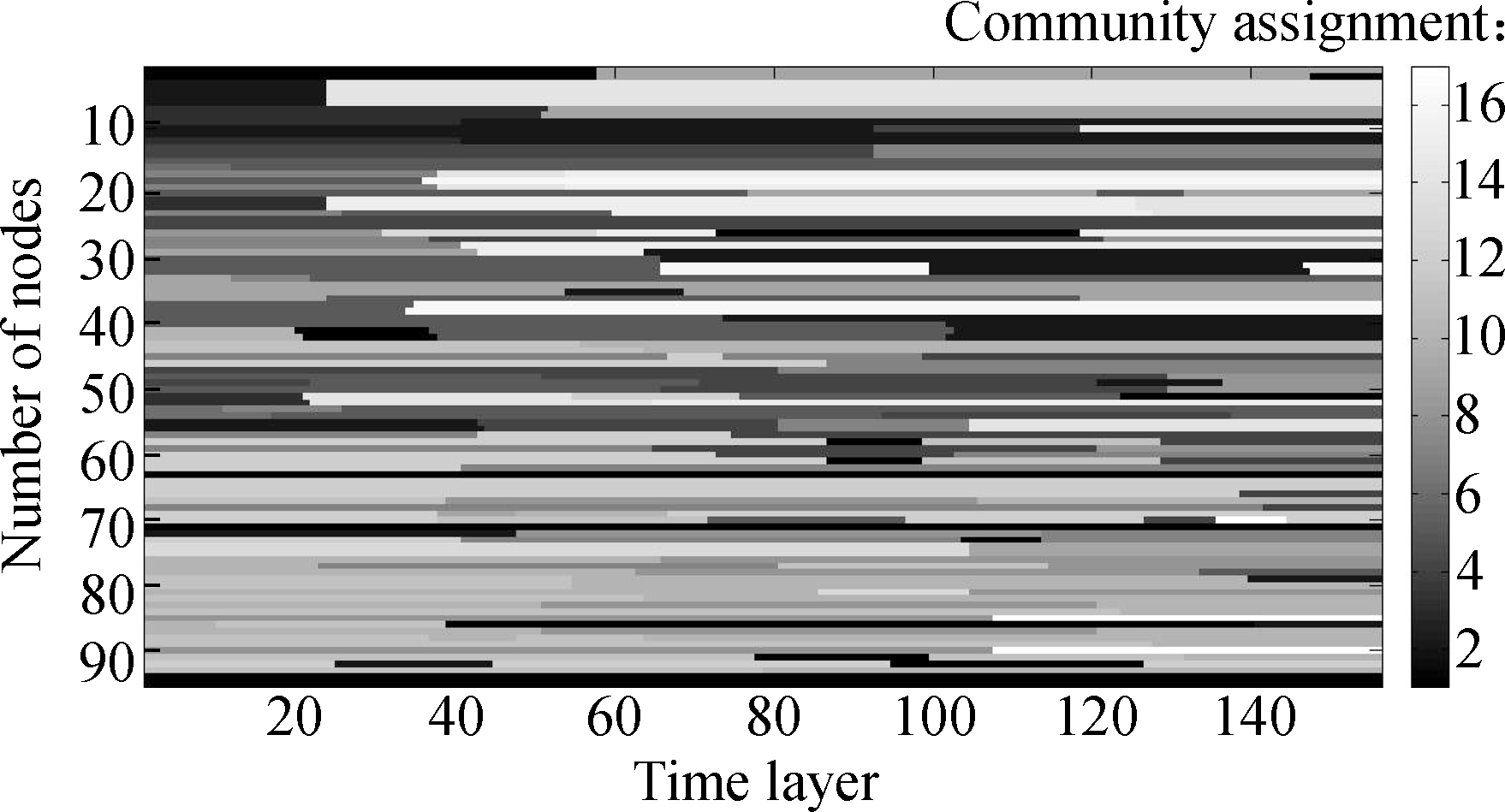
Fig.2 Community assignment of a participant
Tab.2 Results of the flexibility’s pair permutation test

BrainnetworksSubcorticalnetworksAuditorynetworksSomatomotornetworksVisualnetworksCognitivecontrolnetworksDefaultnetworksPvalue0.0340.04590.4160.18960.0112∗0.0038∗Note:∗showssignificantdifferenceaftercorrection.
We used the modularity indexQto assess the robustness of the model and detect the differences of the dynamic community architecture between the real and permuted networks for the dynamic network null models by one-sample t-tests. All t-test results are over 10-20and the dynamic network null model is robust for every subject[11].
Flexibility, one of the traits of dynamic community structure, means the normalized number of times a region changes its module allegiance and manifests the dynamic activity of a node[7]. Its values in the cognitive control network and default network decrease in the post-treatment patients. It is suggested that the cognitive control network is related to cognitive functioning and the default-mode network is implicated in spontaneous and self-generated cognition[12-13]. Meanwhile, the two networks’ abnormalities are both concerned with the depressive episodes[12]. The downtrend of their flexibility means a remission of depression and improvement of cognitive functioning, spontaneous and self-generated cognition. Therefore, the study of the dynamic community structure over brain is a feasible way to analyze the treatment of depression.
[1]Chang C, Glover G H. Time-frequency dynamics of resting-state brain connectivity measured with fMRI[J].Neuroimage, 2010,50(1): 81-98. DOI:10.1016/j.neuroimage.2009.12.011.
[2]Bassett D S, Wymbs N F, Porter M A, et al. Dynamic reconfiguration of human brain networks during learning[J].ProceedingsoftheNationalAcademyofSciences, 2011,108(18): 7641-7646. DOI:10.1073/pnas.1018985108.
[3]Wei M B, Qin J L, Yan R, et al. Abnormal dynamic community structure of the salience network in depression[J].JournalofMagneticResonanceImaging, 2017,45(4): 1135-1143. DOI:10.1002/jmri.25429.
[4]Wei M B, Qin J L, Yan R, et al. Association of resting-state network dysfunction with their dynamics of inter-network interactions in depression[J].JournalofAffectiveDisorders, 2015,174: 527-534. DOI:10.1016/j.jad.2014.12.020.
[5]Bassett D S, Porter M A, Wymbs N F, et al. Robust detection of dynamic community structure in networks[J].Chaos:AnInterdisciplinaryJournalofNonlinearScience, 2013,23(1): 013142. DOI:10.1063/1.4790830.
[6]Yan C G, Zang Y F. DPARSF: A Matlab toolbox for “pipeline” data analysis of resting-state fMRI[J/OL].FrontSystNeurosci, 2010. https://www.ncbi.nlm.nih.gov/pmc/articles/PMC2889691/. DOI:10.3389/fnsys.2010.00013.
[7]Beckmann C F, Mackay C E, Filippini N, et al. Group comparison of resting-state FMRI data using multi-subject ICA and dual regression[J].Neuroimage, 2009,47(Sup 1): S148. DOI:10.1016/s1053-8119(09)71511-3.
[8]Wei M B, Qin J L, Yan R, et al. Identifying major depressive disorder using Hurst exponent of resting-state brain networks[J].PsychiatryResearch:Neuroimaging, 2013,214(3): 306-312. DOI:10.1016/j.pscychresns.2013.09.008.
[9]Allen E A, Damaraju E, Plis S M, et al. Tracking whole-brain connectivity dynamics in the resting state[J].CerebCortex, 2014,24(3): 663-676. DOI:10.1093/cercor/bhs352.
[10]Marrelec G, Krainik A, Duffau H, et al. Partial correlation for functional brain interactivity investigation in functional MRI[J].Neuroimage, 2006,32(1): 228-237. DOI:10.1016/j.neuroimage.2005.12.057.
[11]Mucha P J, Richardson T, Macon K, et al. Community structure in time-dependent, multiscale, and multiplex networks[J].Science, 2010,328(5980): 876-878. DOI:10.1126/science.1184819.
[12]Mulders P C, van Eijndhoven P F, Schene A H, et al. Resting-state functional connectivity in major depressive disorder: A review[J].Neuroscience&BiobehavioralReviews, 2015,56: 330-344. DOI:10.1016/j.neubiorev.2015.07.014.
[13]Dutta A, McKie S, Deakin J F W. Resting state networks in major depressive disorder[J].PsychiatryResearch:Neuroimaging, 2014,224(3): 139-151. DOI:10.1016/j.pscychresns.2014.10.003.
References
摘要:为了更有效地评估抑郁症患者治疗前后的改善效果,使用动态模块化算法探测抑郁症患者静息态脑网络的灵活度属性.使用独立成分分析获得每个被试的特定脑网络分区信号,通过滑动窗口和L1范数计算动态功能连接矩阵,然后运用社区探测算法计算功能连接的动态社区结构.最终获得的模块化分配结构具有大脑活动随时间推移的一般特征.灵活性指标是动态社区结构的特征之一,表征区域变化的次数.本次研究中,有16名患者实现临床缓解并治疗前后各扫描一次.计算得到的所有患者治疗前后全脑6个网络的灵活度指标组间置换检验结果显示,患者治疗前和治疗后的默认网络和认知控制网络灵活性度分布存在下降趋势,且该趋势具有统计学差异.因此这2个网络的灵活度指标可用于抑郁病人治疗效果评估的客观参考.
关键词:动态社区结构;核磁共振成像;抑郁症;治疗效果
中图分类号:TP3
![]()
JournalofSoutheastUniversity(EnglishEdition) Vol.33,No.3,pp.277⁃285Sept.2017 ISSN1003—7985
DOI:10.3969/j.issn.1003-7985.2017.03.004
Foundationitems:The National High Technology Research and Development Program of China (863 program) (No.2015AA020509), the National Natural Science Foundation of China (No.81571639, 81371522, 61372032).
Citation:Mo Zhaoqi, Wang Qiang, Tian Shui, et al. Evaluating treatment via flexibility of dynamic MRI community structures in depression[J].Journal of Southeast University (English Edition),2017,33(3):273-276.
DOI:10.3969/j.issn.1003-7985.2017.03.004.