
Abstract:A theoretical sensitivity analysis of total lost time and saturated flow rate is conducted based on the method proposed in the Highway Capacity Manual (HCM). In addition, the accuracy of the timing calculation algorithm suggested in the HCM is verified using field data from three intersections. It is demonstrated that there is a positive correlation between the estimation error rates of the signal cycle length and the phase lost time. Also, the estimated value of saturated flow rate must meet the specific requirements under different saturated conditions to guarantee the accuracy of the signal cycle length. However, through analysis of field data collected on the discharge headway in three intersections, it is also found that, if the 4th vehicle is set as the initial spot for the stable discharge headway, as is recommended in the HCM, the error of the phase lost time will be over 40% when the line length is over 10 vehicles. Moreover, the calculation error for signal cycle length is not guaranteed to fall within the 15% range when the length of line is over 15 vehicles. It is suggested that, to improve the applicability of the HCM method, a more accurate description of the distributed regularity of the discharge headway is necessary when calibrating key parameters.
Keywords:lost time; saturated flow rate; sensitivity analysis; signal timing
A reasonable signal timing plan is necessary to guarantee the efficiency of an urban transportation network. To optimize a signal timing plan, it is necessary to study methods for enhancing the accuracy and reliability of isolated intersection control. Classic algorithms for signal timing include the British TRL method, the ARRB method, and the method proposed by HCM[1]. The most widely used signal timing algorithm in China is the method proposed in the HCM, which will be used as the foundation for this study to optimize the signal cycle length algorithm.
Classic algorithms generally pay more attention to refining external conditions or set some specific goals. Research on improving classic algorithms was mainly carried out in 1990s, such as the studies of Al-Salman et al.[2]and Yang et al[3]. In recent years, less research on this direction has been done. With the rise of ITS technology, treating signal timing plans as an optimal control problem became a popular new research idea[4]. Fuzzy control, neural networks, and reinforcement learning came to occupy the predominant position. Related studies on intelligent methods can be found in Refs.[5-7] and so on.
Besides improvement on the classic algorithms and intelligent control methods, parameters calibration is an important way to improve the signal control efficiency[8]. Based on Refs.[9-10], it is easy to see that the discharge headway is correlated to the queue position. Saturation flow rate and lost time are computed based on the headway of one specified queue position, which is regarded as the beginning of the saturated flow. However, Shao et al.[11]and some other researchers also show that using the average value of headways statistics to calculate the SFR may result in underestimations. Above all, the importance of parameters calibration for signal timing is obvious while the criterion and acceptable error level for calibration is lacking research.
Based on the errors existing in parameters calibration, this paper performs the sensitivity analysis of the lost time and saturation flow rate. An acceptable error range for calibration is determined, which is useful for evaluating the efficiency of the calibration method.
This study uses the signal timing method recommended in HCM 2010 to perform a sensitivity analysis of the algorithm’s main parameters.
1.1 Calculation method of signal cycle length in HCM
Based on the Highway Capacity Manual 2010, the fundamental theory of signal cycle length calculation can be presented as follows.
The established principle for a signal cycle is that all vehicles can pass through the intersection within the cycle, which means no stranded vehicles. Consequently, the cycle length should be equal to the sum of the lost time of critical phases in one cycle and the time that all arriving vehicles need to pass through the intersection at the saturation state; that is
(1)
whereCis the cycle length, s;Lis the cycle lost time, s;qi/Siis the flow ratio of the critical phaseiin the critical lane;qiis the real arrival flow rate of the critical phase in the critical lane, veh/h;Siis the saturation flow rate of the critical phase in the critical lane, veh/h;nis the number of critical phases.
The arrangement of the above formula can be shown as
C=![]()
(2)
(3)
Y=![]()
(4)
CS=∑CV
(5)
RS=0.9s0PHFfa
(6)
whereYis the sum of the flow ratio of the critical phases;ciis the set of critical phases on the critical path, s;lt,iis the phaseilost timelt,i=l1,i+l2,i;l1,iis the startup lost time,l1,i=2.0 s;l2,iis the clearance lost time,l2,i=A+Rc-e,Ais the yellow change interval, s,Rcis the red clearance interval, s,eis the extension of effective green,e=2.0;CSis the critical sum, veh/h;RSis the reference sum flow rate, veh/h;CVis the critical phase volume, veh/h;PHFis the peak hour factor;s0is the basic saturation flow rate in each lane, pcu/(h·ln);fais the adjustment factor for area type, which is 0.90 for a central business district and 1.00 otherwise.
1.2 Parameter calibration method
According to the signal cycle timing method in HCM 2010, the cycle lost timeLand the sum of the flow ratio of the critical phasesYare two main parameters influencing the accuracy of cycle length estimation.
1.2.1 Calibration of cycle lost time L
As shown in Eq.(3), cycle lost timeLis the sum of the phaseilost time, and the phaseilost time is divided into two parts: start-up lost time and clearance lost time.
It is noted in HCM that the influence of reaction time and acceleration time on traffic flow decreases with vehicles going through the stop line. Supposing that their influence can be ignored when the (m+1)-th vehicle reaches the stop line, the lost time of phaseican be observed and calculated by

(7)
wheretjis the start-up lost time of thej-th vehicle;mis them-th vehicle in the queue.
It is proposed in HCM that the value ofmis 4 under observable situation, and headways after the 4th vehicle can be regarded as stable; under unobservable situations, it is recommended that the start-up lost time of one phase is set to be 2 s.
Clearance lost time can be determined by subtracting the yellow change interval and the extension of the effective green from the red clearance interval. As recommended in HCM, the extension of effective green is 2 s.
1.2.2 Calibration of the sum of flow ratio of critical phase Y
As shown in Eq.(4), the sum of the flow ratio of critical phaseYis the ratio of the critical sumCSto the reference sum flow rateRS. The accuracy ofCSis determined by the precision of the traffic monitoring method, which is not within the research scope in this study; thus,CSis assumed to be accurate.
According to Eq.(6), the reference sum flow rate is composed of the basic saturation flow rate, the peak hour factor, and the adjustment factor for the area type. It should be noted that the basic saturation flow rate is the maximum flow rate under the assumption that the green ratio is equal to 1.0. The value of the basic saturation flow rate can be gathered through a field survey. Also, the rate in each lane is the expected flow rate in a straight vehicle lane in the situation that the adjustment factor is equal to 1.0.
s0=![]()
(8)
wherehis the saturation headway, s.
As pointed out in HCM, when the saturation headway cannot be observed, the default value of the basic saturation flow rate is 1 900 pcu/(h·ln) in metropolitan areas where the population is greater than 250 000 people, and 1 750 pcu/(h·ln) elsewhere.
In order to guarantee the accuracy of signal timing, this study analyzes the lost time and the saturation flow rate, which are two key parameters in the signal timing algorithm.
2.1 Sensitivity analysis of lost time
In ideal circumstances, the signal cycle length can be calculated via Eq.(2) and the parametersLandYcan be determined accurately. However, errors exist in the calibration ofLandYin practical applications. If assuming thatYcan be calibrated accurately and the error exists while calibratingL, the signal cycle length can be calculated as
Ce=![]() =
=![]()
![]() =C
=C![]() =CγL
=CγL
(9)
whereCeis the calculated value of the signal cycle length;Leis the actual calibrated value of lost time;γLis the ratio of actual calibrated value to the theoretical value of lost time (the theoretical value is the calibrated value with no errors).
Therefore, the ratio of the calculated valueCeto the ideal valueCis represented as
![]() =γL
=γL
(10)
It is illustrated here that there is a positive correlation between the error of the total lost time and that of the calculated value for the signal cycle length. As Eq.(3) shows, the total lost time is the sum of the lost time in each phase, which includes the start-up lost time and the clearance lost time. It can be concluded that the total lost time of a signal cycle is influenced by the number of phases, the start-up lost time, and the clearance lost time.
In the application of signal control in China, the most commonly used signal timing plans are two phases, three phases, and four phases. There is no all-red clearance interval. The extension of green time can be set to be 2 s as recommended in HCM, and the clearance lost time for each phase is 1 s. It is proposed in HCM that the start-up lost time can be 2 s for each phase when there is no survey data. However, it is believed that this value has a relatively large error and cannot be adopted without appropriate research. Therefore, the total lost time of the signal cycle length can be generated as
(11)
So the total lost time of the signal timing plan depends on the number of phases and the start-up lost time. As there are no effects on the analysis results, it can be assumed that using the same method for lost time estimation leads to the same estimation error for each phase. The error in the total lost time remains on the same scale as the error in each phase; that is, the scales of the errors for total lost time and forl1,i+1 are the same.
In accordance with Eq.(10), the ratio of the calculation error for the signal cycle length is positively related to the ratio of the lost time error as well as the ratio of error forl1,i+1. When it is required that the error for the signal cycle length calculation is no more than 5%, 10%, or 15%, the estimation error forl1,i+1 in each phase should be no more than 5%, 10%, or 15%, respectively.
2.2 Sensitivity analysis of saturation flow rate
If assuming thatLcan be calibrated accurately, and error exists when calibratingY, then the calculation result for the signal cycle length can be established as
Ce=![]() =
=![]() =
= =
=![]()
(12)
whereYeis the calibrated value of the sum of the flow ratio of the critical phases;RSeis the actual calibrated value of the reference sum flow rate;γQis the ratio of the actual calibrated value to the theoretical value of the saturation flow rate (theoretical value is the calibrated value with no errors), andγQ>Y.
It can be concluded from Eq.(12) that, when error exists in the sum of the flow ratio in the critical phasesY, the ratio of the calculated value of the signal cycle lengthCeto the ideal valueCcan be depicted as
dc=![]() =
=![]()
(13)
wheredcis defined as the accuracy of the cycle length.
Fig.1 Three-dimensional function ofγQ,Y, anddc
As illustrated in Fig.1,dcis significantly influenced by the valuesYandγQ, and as the value ofYincreases, the sensitivity ofdctoγQincreases. As the accuracy of the cycle lengthdcmust be guaranteed to meet the overall objective of signal timing, the requirements ofγQfor intersections under different levels of saturation are important.
Engineering applications require the calculation error of signal cycle length to be as small as possible. However, although it is impossible to be completely accurate, it is possible to control the error scale within an acceptable range, e.g., 5%, 10%, or 15%. The acceptable ranges fordccorresponding to the error ranges of 5%, 10%, and 15% are 0.95≤dc≤1.05, 0.90≤dc≤1.10, and 0.85≤dc≤1.15, respectively, and the requirements forYandγQare as
0.95≤dc≤1.05, ![]() ≤γQ≤
≤γQ≤![]() (14)
(14)
0.90≤dc≤1.10, ![]() ≤γQ≤
≤γQ≤![]() (15)
(15)
0.85≤dc≤1.15, ![]() ≤γQ≤
≤γQ≤![]() (16)
(16)
Signal control is usually performed at intersections with a relatively large flow rate, and no signal control intersections typically operate under small saturation. Therefore, Eqs.(14) to (16) are suitable for intersections whose saturation is greater than 0.15. According to Eqs.(14) to (16), for intersections under different saturations,γQmust meet the requirements listed in Tab.1 to guarantee the required level of accuracy for the signal cycle length. For example, when an intersection is under the saturation of 0.6 and it is required that the calculation error of the signal cycle length is less than 10%, then the value ofγQmust fall within the range of [0.94,1.08].
Tab.1 The range ofγQat different levels of accuracy for signal cycle length of intersections at different saturations
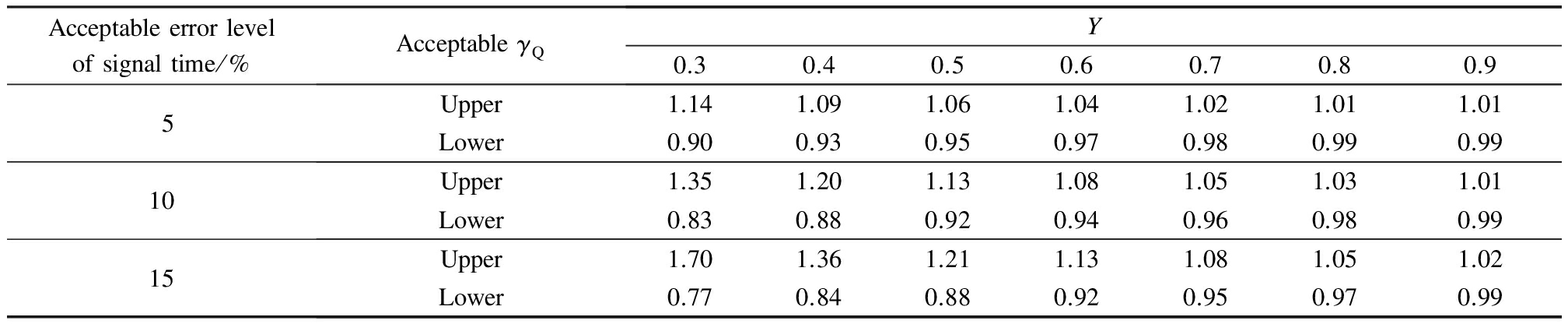
Acceptableerrorlevelofsignaltime/%AcceptableγQY0.30.40.50.60.70.80.95Upper1.141.091.061.041.021.011.01Lower0.900.930.950.970.980.990.9910Upper1.351.201.131.081.051.031.01Lower0.830.880.920.940.960.980.9915Upper1.701.361.211.131.081.051.02Lower0.770.840.880.920.950.970.99
3.1 Basic data collection
Three intersections in Nanjing, China, are selected for collection of headway. The field study focuses on through traffic during morning peak (7:30—8:30) and evening peak (17:00—19:00) on weekdays. One through lane is chosen for each intersection. Recorded videos are processed manually. For the first vehicle of a queue, the discharge headway is the elapsed time between the start of a green light and the time when the vehicle’s front bumper passed the stop line. For the remaining vehicles, including all vehicles that join the queue during the green, the discharge headways are the elapsed time between the points when two successive vehicles’ front bumpers pass the same stop line.
The headway is collected in groups; each group contains the headways for all vehicles in the queue for one phase. The numbers of valid headway data for the three intersections are 301, 302, and 320. All data is presented in Tab.2. The headway at each spot in line is the average of valid data. The saturation flow rate at that spot can be calculated according to Eq.(8).
Tab.2 Statistical parameters for entering headway
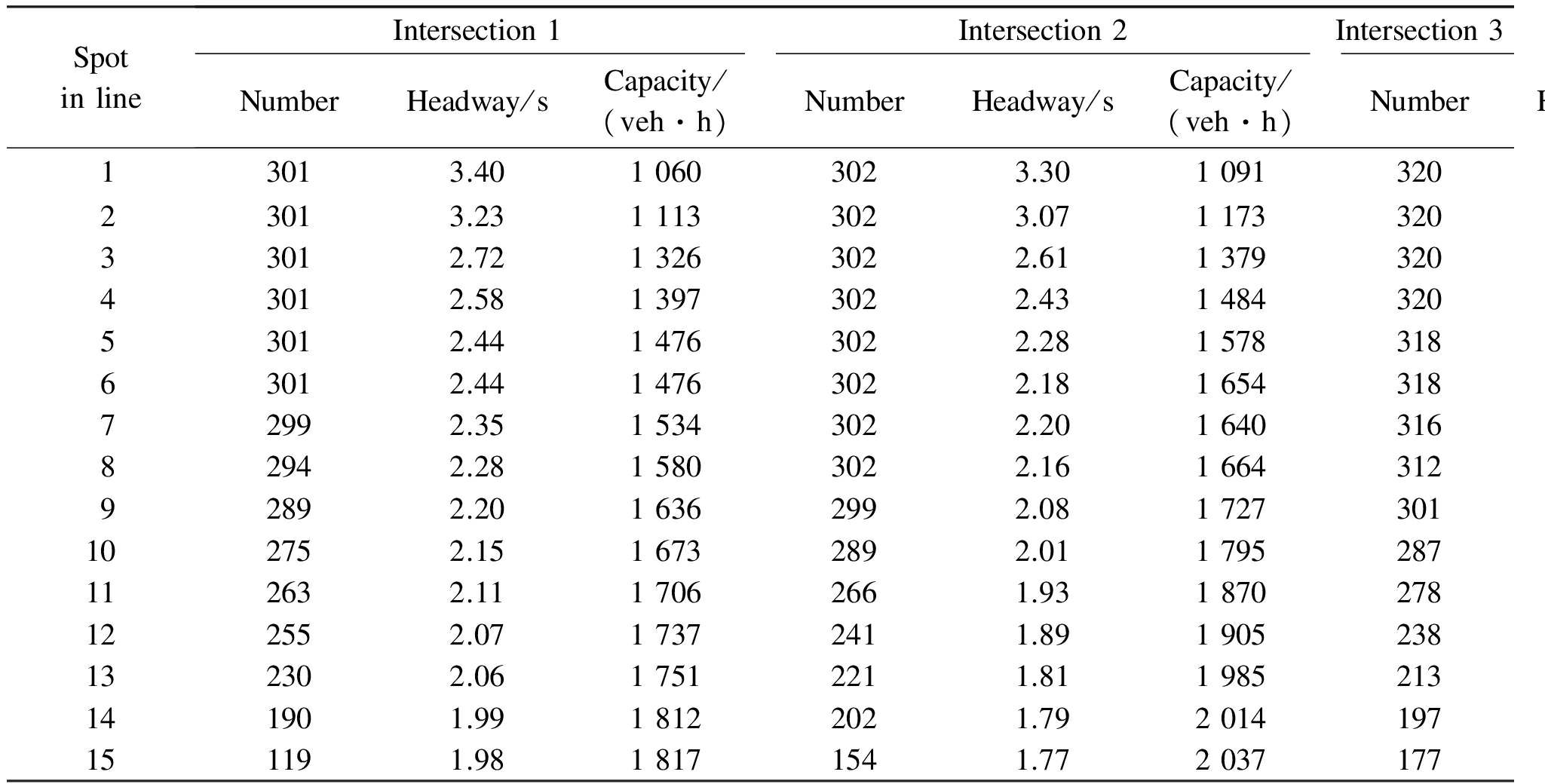
SpotinlineIntersection1Intersection2Intersection3NumberHeadway/sCapacity/(veh·h)NumberHeadway/sCapacity/(veh·h)NumberHeadway/sCapacity/(veh·h)13013.4010603023.3010913203.8793023013.2311133023.0711733203.44104733012.7213263022.6113793203.00120143012.5813973022.4314843202.68134153012.4414763022.2815783182.60138363012.4414763022.1816543182.60138772992.3515343022.2016403162.49144482942.2815803022.1616643122.44147692892.2016362992.0817273012.431484102752.1516732892.0117952872.261591112632.1117062661.9318702782.231612122552.0717372411.8919052382.221624132302.0617512211.8119852132.111705141901.9918122021.7920141972.081731151191.9818171541.7720371772.061750
3.2 Accuracy analysis for total lost time calibration
According to the sensitivity analysis of lost time, the ratios of calculation error for the signal cycle length and the error ofl1,i+1 are positively related. It is stated in HCM that the discharge headway will remain stable after the 4th vehicle, meaning that the start-up lost time can be set to be 2 s when it is unobservable.
For the data from three intersections, each spot between the 4th and the 15th vehicle is set as an assumed stable spot for discharging vehicles in the queue and the value ofl1,i+1 is calculated. Results are shown in Tab.3.
Tab.3 Lost time analysis of queuing vehicles achieving stable conditions at different spots in line
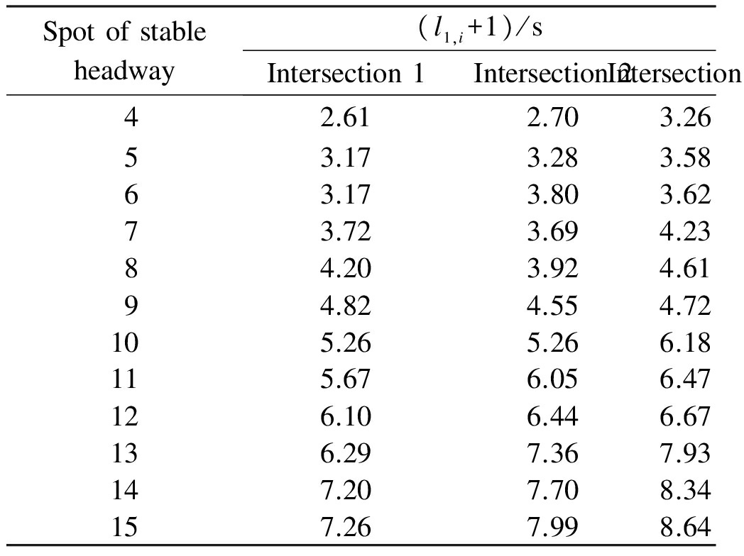
Spotofstableheadway(l1,i+1)/sIntersection1Intersection2Intersection342.612.703.2653.173.283.5863.173.803.6273.723.694.2384.203.924.6194.824.554.72105.265.266.18115.676.056.47126.106.446.67136.297.367.93147.207.708.34157.267.998.64
If it is assumed that the discharge headway achieves a stable condition after the 4th vehicle, the values ofl1,i+1 for the three intersections are, respectively, 2.61, 2.70, and 3.26 s. If it is considered that the discharge headway achieves a stable condition after the 10th vehicle, the values ofl1,i+1 are, respectively, 5.20, 5.26, and 6.18 s. It is obvious that the values ofl1,i+1 under the latter assumption are greater than 90%, which are larger than those under the former assumption. Moreover, the values ofl1,i+1 under the assumption that the discharge headway achieves a stable condition after the 15th vehicle are greater than 40%, which are larger than those under the assumption that the stable spot is at the 10th vehicle. The ratios of calculation error for the signal cycle length when assuming that the saturated spots of the discharge headway are at the 4th, 10th, and 15th vehicle are thus over 40%, and even over 90%. Therefore, it can be concluded that it is not appropriate to set the spot of the 4th vehicle as the initial saturation point for the discharge headway, and the changes in headways at a subsequent spot in line have a significant influence on the calculation of signal cycle length.
3.3 Accuracy analysis for saturation flow rate calibration
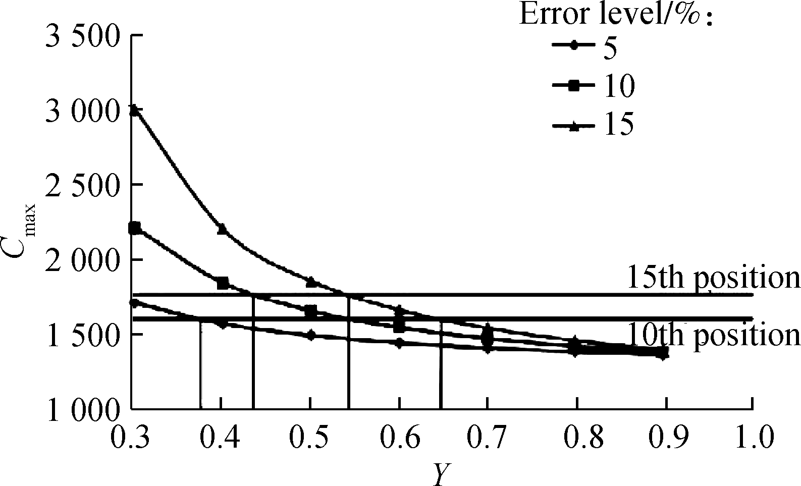
If the discharge headway is stable after the 4th vehicle, the saturation flow rates of the three intersections can be obtained by Tab.2, and these are, respectively, 1 397, 1 484, and 1 341 veh/h. To ensure that the error rate of the signal cycle length is within the range of 5%, 10%, or 15%, the acceptable maximum values for the real saturation flow rate can be calculated by
Cmax=![]() γQU
γQU
(17)
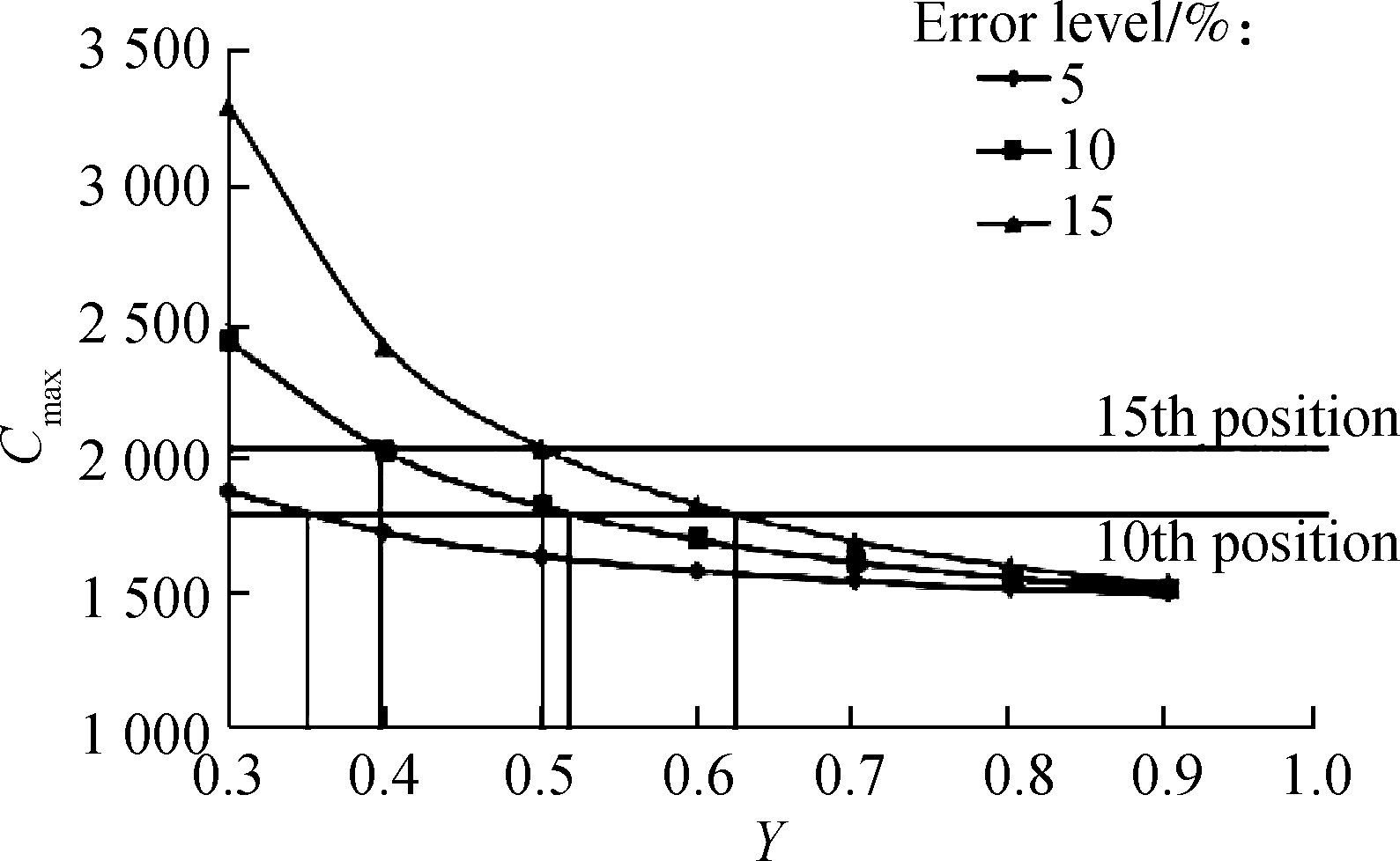
whereCmaxis the acceptable maximum value of the real saturation flow rate;C4this the saturation flow rate at the spot in line of the 4th vehicle;γQUis the acceptable upper bound ofγQin 0;γQLis the acceptable lower bound ofγQin 0. These calculation results are shown in Fig.2.
Fig.2 illustrates that, when the calculation error for signal cycle length falls within 5%, the saturation flow rate at the 10th vehicle is over the value ofCmaxat most levels of saturation. When the calculation error for the signal cycle length is required to be within 10%, the value ofCmaxunder a saturation of over 0.55 is lower than the saturation flow rate at the spot of the 10th vehicle, and theCmaxunder a saturation over 0.45 is lower than the saturation flow rate at the spot of the 15th vehicle. When the calculation error for the signal cycle length is required to be within 15%, theCmaxfor saturation over 0.55 is lower than the saturation flow rate at the spot of the 15th vehicle. Also, as was proven, the results of this analysis are the same when the spot of the 6th vehicle or the 8th vehicle is set as the initial spot of saturation.

(a)
(b)
(c)
Fig.2 Acceptable maximum values of real saturation flow rateCmaxunder different conditions. (a) Intersection 1; (b) Intersection 2; (a) Intersection 3
It can thus be concluded that, when the spot in the line of the 4th vehicle is used as the initial spot for the stable discharge headway, the saturation flow rates at the spot of the 10th and 15th vehicles are over the value ofCmaxat most saturations. Particularly when the intersections are at a high level of saturation, the real saturation flow rates in the subsequent spots are over the acceptable maximum saturation flow rate when the 4th vehicle is set as the initial spot of stabilization. The desired accuracy in signal cycle length cannot be guaranteed even when setting the spot of the 6th or 8th vehicle as the initial stable spot of the discharge headway.
1) There is a positive correlation between the value ofl1,i+1 and the error rate of the calculated result for the signal cycle length. The error ofl1,i+1 is large when different spots in line are set as the initial stable spot of the discharge headway.
2) It is found thatγQandYshould obey a specific relationship to guarantee the calculation error for signal cycle length within a desired accuracy level. The relationship indicates that theγQvalue must be within specified ranges under different saturations.
3) It is suggested that the calibration ofLandRSmust meet specific requirements to guarantee the accuracy of calculating signal cycle length. As a result of limited field data, the initial stable spot for the discharge headway is not clear. However, it is important to precisely calibrate the regularity of the discharge headway to improve the accuracy of signal timing.
[1]National Research Council. Highway capacity manual (HCM2010)[S]. Washington, DC, USA: Transportation Research Board, 2010.
[2]Al-Salman H, Salter R J. Control of right-turning vehicles at signal-controlled intersections[J].TrafficEngineeringandControl, 1974,15(15): 683-686.
[3]Yang P, Yang S.Trafficmanagementandcontrol[M]. Beijing: China Communications Press, 1995: 135-147. (in Chinese)
[4]Kamien M I, Schwartz N L.Dynamicoptimization:Thecalculusofvariationsandoptimalcontrolineconomicsandmanagement[M]. Chelmsford: Courier Corporation, 2012: 203-209.
[5]Shirvani M J, Maleki H R. Maximum green time settings for traffic-actuated signal control at isolated intersections using fuzzy logic[J].InternationalJournalofFuzzySystems, 2017,19(1): 247-256. DOI:10.1007/s40815-016-0143-7.
[6]Cui C, Kui Z, Lee H, et al. Offset control of traffic signal using cellular automaton traffic model[J].ArtificialLifeandRobotics, 2017,22(2): 145-152. DOI:10.1007/s10015-017-0356-3.
[7]Eriskin E, Karahancer S, Terzi S, et al. Optimization of traffic signal timing at oversaturated intersections using elimination pairing system[J].ProcediaEngineering, 2017,187: 295-300. DOI:10.1016/j.proeng.2017.04.378.
[8]Yang X, Zhuang B, Li K. Analysis of saturation flow rate and delay at signalized intersection [J].JournalofTongjiUniversity(NaturalScience), 2006,34(6): 738-743. (in Chinese)
[9]Bagheri E, Mehran B, Hellinga B. Real-time estimation of saturation flow rates for dynamic traffic signal control using connected-vehicle data[J].TransportationResearchRecord:JournaloftheTransportationResearchBoard, 2015,2487: 69-77. DOI:10.3141/2487-06.
[10]Shang H, Zhang Y, Fan L. Heterogeneous lanes’ saturation flow rates at signalized intersections[J].Procedia-SocialandBehavioralSciences, 2014,138: 3-10. DOI:10.1016/j.sbspro.2014.07.175.
[11]Shao C Q, Rong J, Liu X M. Study on the saturation flow rate and its influence factors at signalized intersections in China[J].Procedia—SocialandBehavioralSciences, 2011,16: 504-514. DOI:10.1016/j.sbspro.2011.04.471.
References
摘要:以HCM提出的信号配时算法为基础,对总损失时间和饱和流率的敏感度进行了理论分析.利用3个交叉口的实地采集数据对HCM推荐的信号配时算法的准确性进行了验证.结果表明,信号周期时长的估算误差率和相位损失时间的估算误差率成正比.同时,为保障信号周期的预测精度,在不同的饱和条件下,饱和流率的估算值必须满足特定的要求.通过对3个交叉口车头时距数据的分析发现,若根据HCM的建议将第4辆车作为饱和车头时距标定的起点,则排队长度超过10辆车时总损失时间的误差高达40%,且排队长度大于15辆车时信号周期时长的计算误差很难小于15%.为提高HCM的实用价值,建议在对核心参数进行标定时对车头时距的分布规律进行更精确的描述.
关键词:损失时间;饱和流率;敏感度分析;信号配时
中图分类号:U121
![]()
JournalofSoutheastUniversity(EnglishEdition) Vol.33,No.3,pp.322⁃329Sept.2017 ISSN1003—7985
DOI:10.3969/j.issn.1003-7985.2017.03.010
Foundationitems:Jiangsu Science and Technology Project (No.BY2016076-05), the Scientific Research Foundation of Graduate School of Southeast University, the Fundamental Research Funds for the Central Universities, the Scientific Innovation Research of College Graduates in Jiangsu Province (No. KYLX15_0152).
Citation:Zhao Yi, Zhong Ning, Lu Jian, et al. Analysis of key parameters sensitivity and calibration accuracy of signal timing algorithm[J].Journal of Southeast University (English Edition),2017,33(3):316-321.
DOI:10.3969/j.issn.1003-7985.2017.03.010.