
(a) (b)
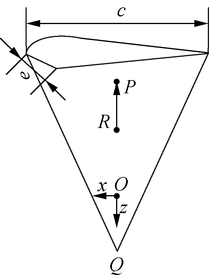
Fig.1 The schematics of the parafoil canopy. (a) The front view; (b) The side view
Abstract:In order to better study the dynamic characteristics and the control strategy of parafoil systems, considering the effect of flap deflection as the control mechanism and regarding the parafoil and the payload as a rigid body, a six degrees-of-freedom (DOF) dynamic model of a parafoil system including three DOF for translational motion and three DOF for rotational motion, is established according to the Kirchhoff motion equation. Since the flexible winged parafoil system flying at low altitude is more susceptible to winds, the motion characteristics of the parafoil system with and without winds are simulated and analyzed. Furthermore, the airdrop test is used to further verify the model. The comparison results show that the simulation trajectory roughly overlaps with the actual flight track. The horizontal velocity of the simulation model is in good accordance with the airdrop test, with a deviation less than 0.5 m/s, while its simulated vertical velocity fluctuates slightly under the influence of the wind, and shows a similar trend to the airdrop test. It is concluded that the established model can well describe the characteristics of the parafoil system.
Key words:parafoil system; dynamic modeling and simulation; flight characteristic; airdrop experiment; flap deflection
The parafoil system is a type of flexible wing vehicle, which is made up of a ram-air parafoil canopy and a payload. It is a type of precision aerial delivery system with superior pneumatic performance, excellent gliding ability and easy handling property. It now has been widely used in military, aerospace and civil fields due to its excellent properties[1]. To study the parafoil system, the first task is to explore its basic movement characteristics. Mathematical models of parafoil systems obtained by theoretical analysis can be used for studying its stability and flight performance as well as the design and validation of GNC algorithms[2-3].
In recent decades, researchers have done much exploration of dynamic modeling of parafoil systems. One of the first models was studied by Goodrick[4] who developed a six DOF model to analyze the response to manual and automatic control inputs in 1979. Iacomini and Cerimele[5] explored the lateral and longitudinal aerodynamics for large-scale parafoils from the flight test data of NASA’s X-38 parafoil program. Zhang et al.[6] and Tao et al.[7] used a three DOF motion model of parafoil systems for planning optimal homing trajectories. Barrows[8] mainly focused on the calculations of the apparent mass of parafoils, and presented dynamic equations including nonlinear terms of a six DOF model. Xiong[9] and Jiao et al.[10]also established a six DOF model for trajectory design and homing control. Considering the relative pitch and yaw motion between the parafoil and the payload, Slegers et al.[11-15] applied the concept of coupling of moments between the payload and parafoil at the joining to establish an eight DOF model of parafoil systems. Prakash and Ananthkrishnan[16] and Yu[17] set up a nine DOF dynamic model of parafoil-payload systems, which includes six DOF for the parafoil canopy and the payload, as well as three DOF for the translational motion of the confluence point of the lines.
With the existence of flap deflection in turning and flare landing, aerodynamic performances of the parafoil system greatly differ from the sliding stage, the calculation of which is ignored by most of the existing dynamic models. Flying in a complicated environment, the parafoil system may encounter a sudden gust, which may cause severe impact on its aerodynamic performance, affecting the desired trajectory, even leading to stall. However, the study of the wind field is relatively limited at present. In this paper, considering the effect of flap deflection, a dynamic model of the parafoil system is established based on the Kirchhoff motion equation. The basic motion characteristics of the parafoil system and effects of winds on its aerodynamics performance are simulated and analyzed. The results of simulation and airdrop experiments verify the established dynamic model of the parafoil system.
The schematics of parafoils are shown in Fig.1. The corresponding parameters[8-9] are described as follows: c denotes the length of horizontal projection along the chord; b denotes the length of horizontal projection along the span; e denotes the maximum distance from the upper chord line to the lower chord line along the span; h denotes the distance from the circular arc vertex to the line of two end-points; r denotes the distance from Q to the canopy; Θ denotes half of the central angle of the circular arc canopy. Assuming that Q is the circle center of the circular arc canopy, four important points P, R, O and Q are collinear. P denotes the pitch center; R denotes the roll center; and O denotes the mass center of the parafoil system.
(a) (b)
Fig.1 The schematics of the parafoil canopy. (a) The front view; (b) The side view
In order to facilitate analysis, three main coordinate frames[9,14], as shown in Fig.2, are established and described as follows:
1) Inertial coordinate frame. A fixed point Oe in space is chosen as an inertial coordinate origin. The axis Oeze is vertically downward, and Oexe is located in the horizontal plane and points to the initial motion direction. Oexe is perpendicular to the plane Oexeze.
2) Body coordinate frame. The origin Ob of the body coordinate frame is the mass center of the parafoil system. The axis Obzb is located in the longitudinal symmetry plane of the canopy and points to C. The axis Obxb is perpendicular to the plane and points to the left side of the canopy. The axis Ox is perpendicular to the plane Obxbzb.
3) Wind coordinate frame. The pressure center of the canopy is taken as the origin Oq of the wind coordinate frame. The direction of axis Oqxq is the same as that of wind. The axis Oqzq is located in the longitudinal symmetry plane and points to the lower wing surface. The axis Oqxq and the other two axes constitute a right-handed coordinate frame.
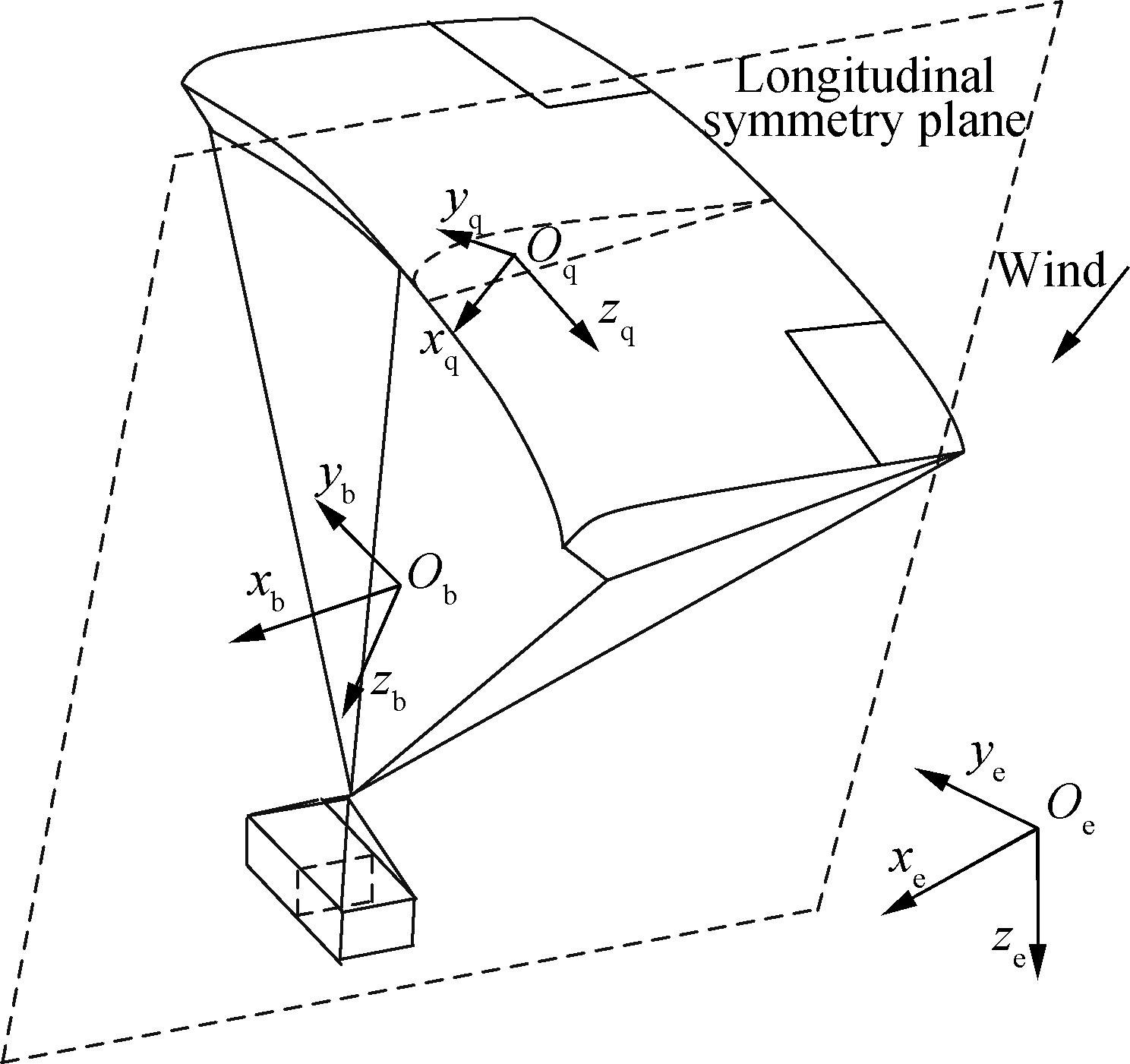
Fig.2 The schematics of the related coordinate frames
Before modeling, three reasonable hypotheses should be made to facilitate analysis[9-10]:
1) After the canopy has been inflated completely, its aerodynamic configuration keeps fixed without maneuvering.
2) The parafoil and payload are regarded as a rigid body, and the mass center of the canopy overlaps the aerodynamic pressure center.
3) The payload is regarded as a revolutionary body, such that the lift of the payload is ignored and only its aerodynamic drag force is considered.
The dynamic equations of the parafoil system can be obtained by the momentum and angular momentum theorem. Considering the fact that the parafoil canopy is made of flexible fabric, the apparent mass must be taken into account and the calculating method was given in Ref.[8]. The quantity of apparent mass is associated with motion directions. However, the traditional rigid body dynamic equations often obscure the changes of the apparent mass under different coordinate frames, which may lead to incorrect results[18]. Accordingly, the Kirchhoff motion equation is applied to describe the dynamic equations of a parafoil system.
The momentum Pr and angular momentum Hr caused by the real mass are expressed as
Pr=mrV
(1)
Hr=JrW
(2)
where V=(u, v, w)T denotes the velocity vector; W=(p, q, r)T represents the angular velocity vector; mr denotes the real mass; and Jr denotes the momentum of the inertia of the real mass.
The corresponding matrix form of Eqs.(1) and (2) can be rewritten as
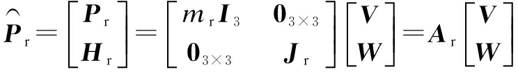
(3)
where Ar denotes the inertia matrix of real mass.
The momentum Pr and angular momentum Ha caused by the apparent mass can be calculated as

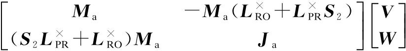
(4)
where Aa denotes the inertia matrix of apparent mass; Ma denotes the apparent mass; Ja denotes the momentum of the inertia of the apparent mass; S2 denotes a choice matrix; LRO=(xRO, yRO, zRO) denotes the vector from R to O, and ![]() is defined as
is defined as ![]() =
= .
.
The total momentum PT and the total angular momentum HT of the whole system in Oxyz can be expressed as

(5)
According to the Kirchhoff motion equation, the motion equations of a parafoil system are expressed as

(6)

W×Hr+V×Pr=Maero+Mex
(7)
where F and M denote the force and the moment, respectively; the subscript aero denotes aerodynamic forces associated with the traditional aerodynamic coefficient and static derivative, and the subscript ex denotes the external force except for the the aerodynamic force, but for parafoil systems, the only external force is gravity.
Faero, Fex, Mearo and Mex in Eqs.(6) and (7) can be written as
Faero=Faero,p+Faero,l+Faero,f
(8)
Fex=FG,p+FG,l
(9)
Maero=Maero,p+Maero,l+Maero,f
(10)
Mex=MG,p+MG,l
(11)
where the subscript G denotes gravity; the subscripts p, l and f denotes the canopy, the payload and the flap, respectively.
Furthermore, Eqs.(6) and (7) can be rewritten as

(12)

(13)
Define
Fr,nl=-W×Pr=-W×mrV
(14)

(15)
Mr,nl= -W×Hr-V×Pr=-W×JrW-V×mrV=
-W×JrW
(16)
Ma,nl= -W×Ha-V×Pr=

(17)
where subscript nl denotes the nonlinear force and moment.
Then, the dynamic model of the parafoil system can be expressed as

(18)
It is clear that the calculation of the aerodynamics of the parafoil is a key step in the modeling progress. Aerodynamic forces acting on the canopy consist of the lift and drag forces of the canopy, and the lift and drag forces of flaps.
2.2.1 Aerodynamic force and moment of canopy
Since the airflow velocity and the angle of attack along the span-wise change dramatically in the progress of turning, and the lift force takes an elliptical distribution in span-wise, therefore, the segmentation method presented by Ref.[4] is used to calculate the aerodynamic forces acting on the canopy. The canopy is divided into eight distributed segments geometrically along the span-wise direction, as shown in Fig.3. The lift coefficient of each segment from outside to inside in turn is multiplied by the factor ki.
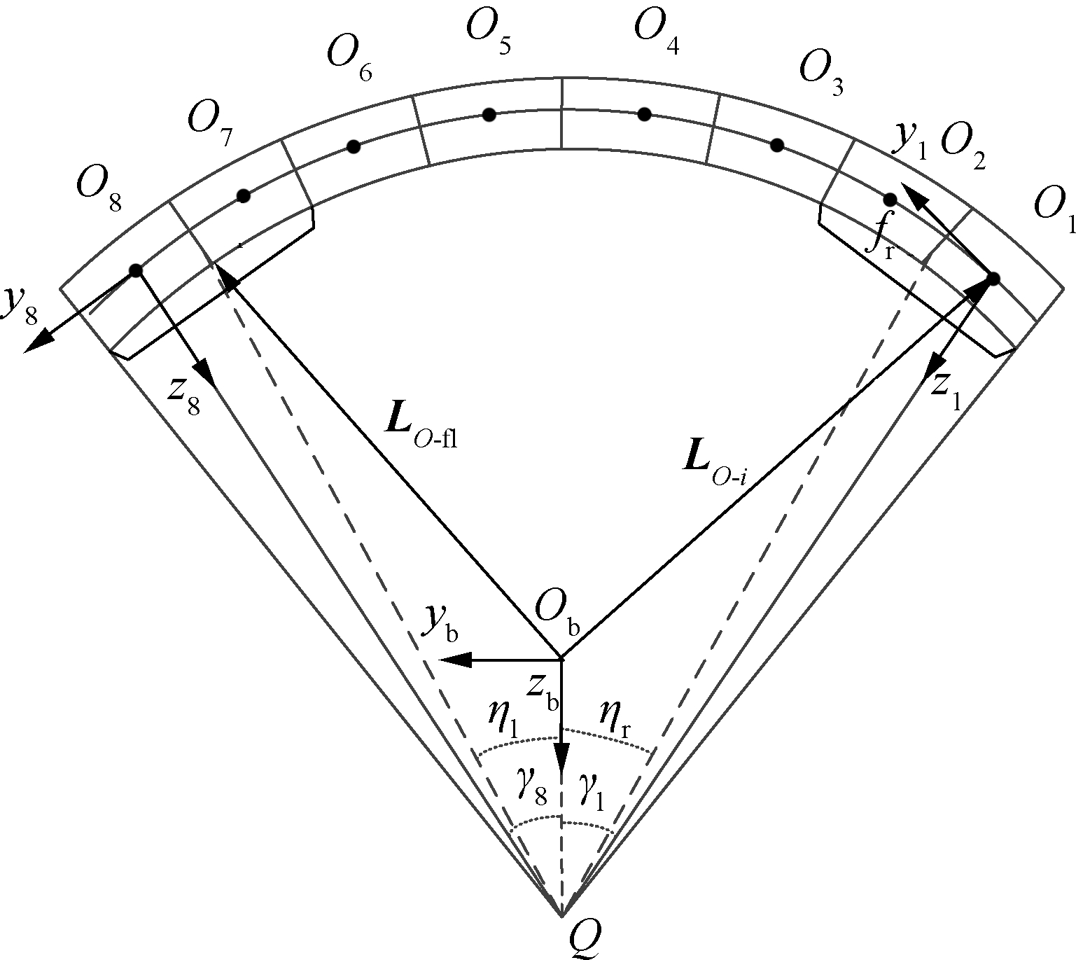
Fig.3 The front view of segmentation
The aerodynamic forces of the i-th segment can be obtained by

(19)

(20)
where the subscript i=1,2,…,8 denotes the serial number of segments; C denotes the aerodynamic coefficient, the subscript L and D denote the lift and drag coefficients, respectively; ρ denotes the density of air; Si denotes the area of the i-th segment; ui, vi and wi denote the velocity vector components of each segment in the i-th coordinate frame.
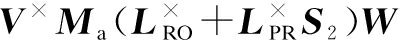
The total aerodynamic force Faero,p and moment Maero,p of canopy with respect to the mass center O are expressed as

(21)
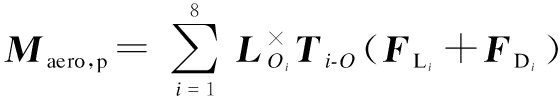
(22)
where Ti-O denotes the transformation from the local coordinate frame of the i-th segment to the body coordinate frame, and can be achieved by rotating γi around the axis xi; ![]() is defined as same as
is defined as same as ![]() in Eq.(4).
in Eq.(4).
2.2.2 Aerodynamic force and moment of flaps
For parafoil systems, flight control is achieved by changing the length of steering lines connected to the outboard side and the rear of the canopy. Pulling down steering lines leads to complex changes in the shape and orientation of the lifting surface. The downward bending of the trailing edge forms the flaps and flap deflection angle.
The aerodynamic forces of flaps are expressed as

(23)

(24)
The total aerodynamic force and moment are expressed as
Faero,f=Tfr-O(FLfr+FDfr)+Tfl-O(FLfl+FDfl)
(25)

(26)
where the subscript fr and fl denote the right and left flap, respectively; the transformation matrix Tfr-O and Tfl-O are defined as same as Ti-O; ![]() and
and ![]() are defined similarly to
are defined similarly to ![]() in Eq.(22).
in Eq.(22).
The simulation experiments are conducted based on a certain type of parafoil systems and physical parameters are listed in Tab.1.
Tab.1 Physical parameters of the parafoil system

ParametersValuesb/m6.2c/m3.6Areaofcanopy/m221.0r/m4.0Riggingangle/(°)10Massofcanopy/kg20Massofpayload/kg80Characteristicareaofpayload/m20.5Characteristicareaofflap/m20.88
The initial values of the model are set as follows: initial position (x, y, z)=(0, 0, 2 000 m); initial velocity (u, v, w)=(15.9 m/s, 0, 2.1 m/s); and initial angular velocity (p, q, r)=(0, 0, 0).
According to the different manipulations of the parafoil system, there are three basic motion patterns, including glide without manipulation, turn with unilateral deflection, and deceleration or flare landing with bilateral deflection.
3.1.1 Gliding
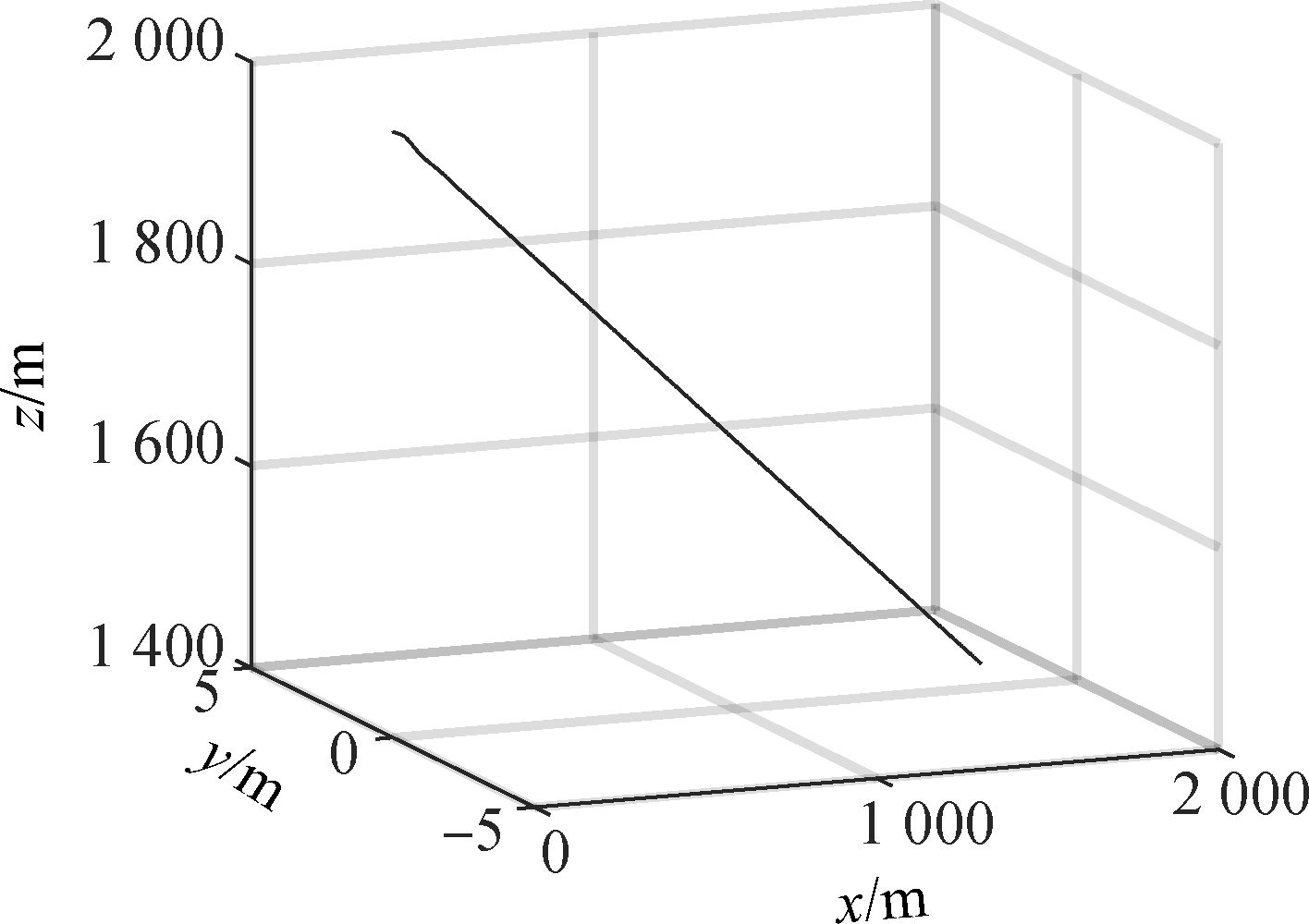
The parafoil system glides with no manipulation. The corresponding motion characteristics are shown in Fig.4.

(a)
(b)
(c)
(d)
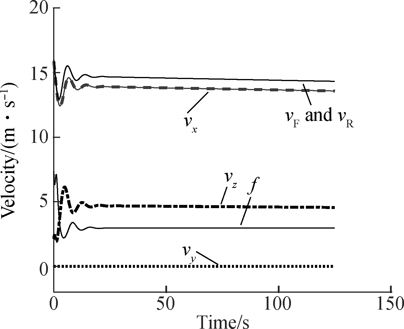
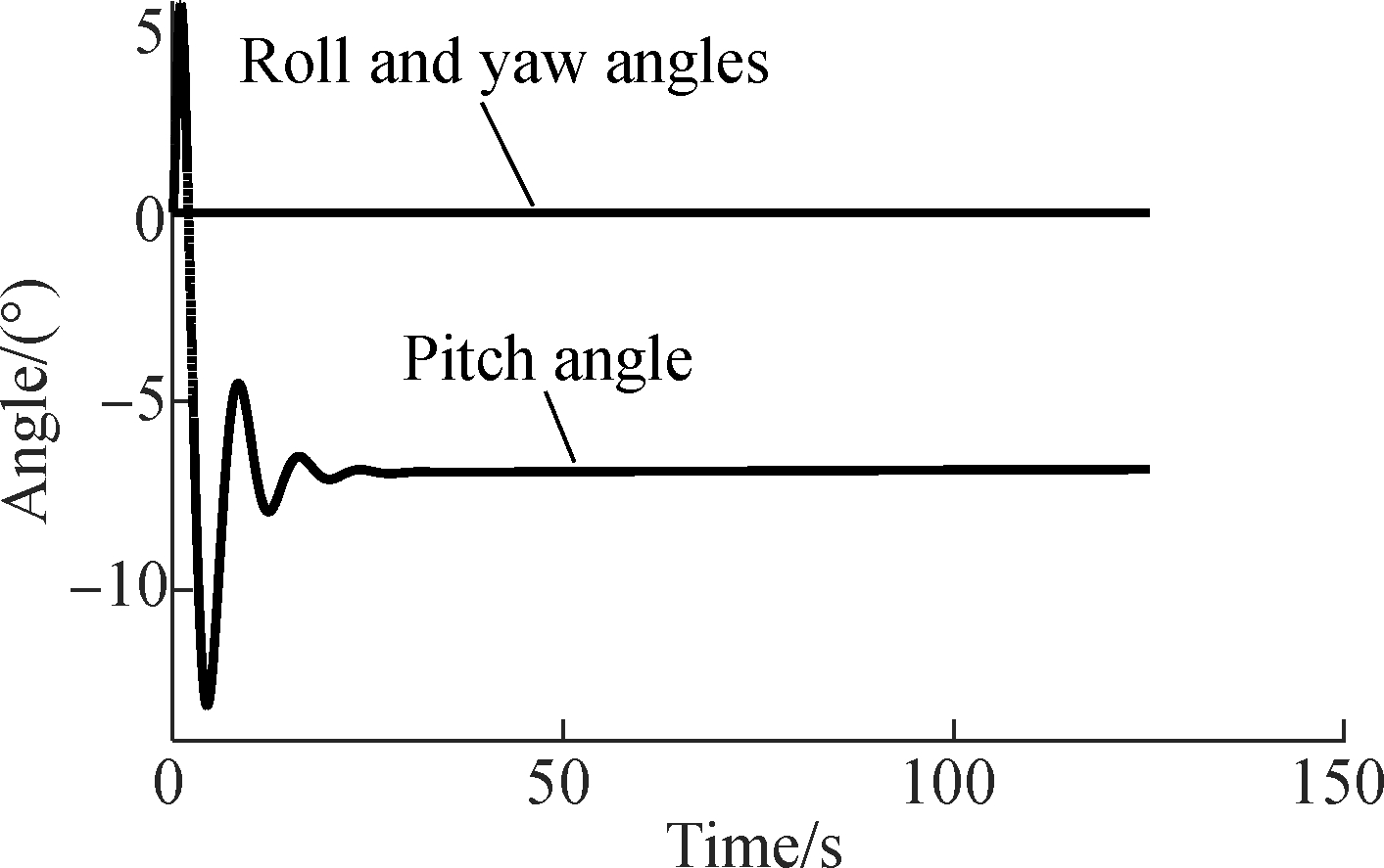
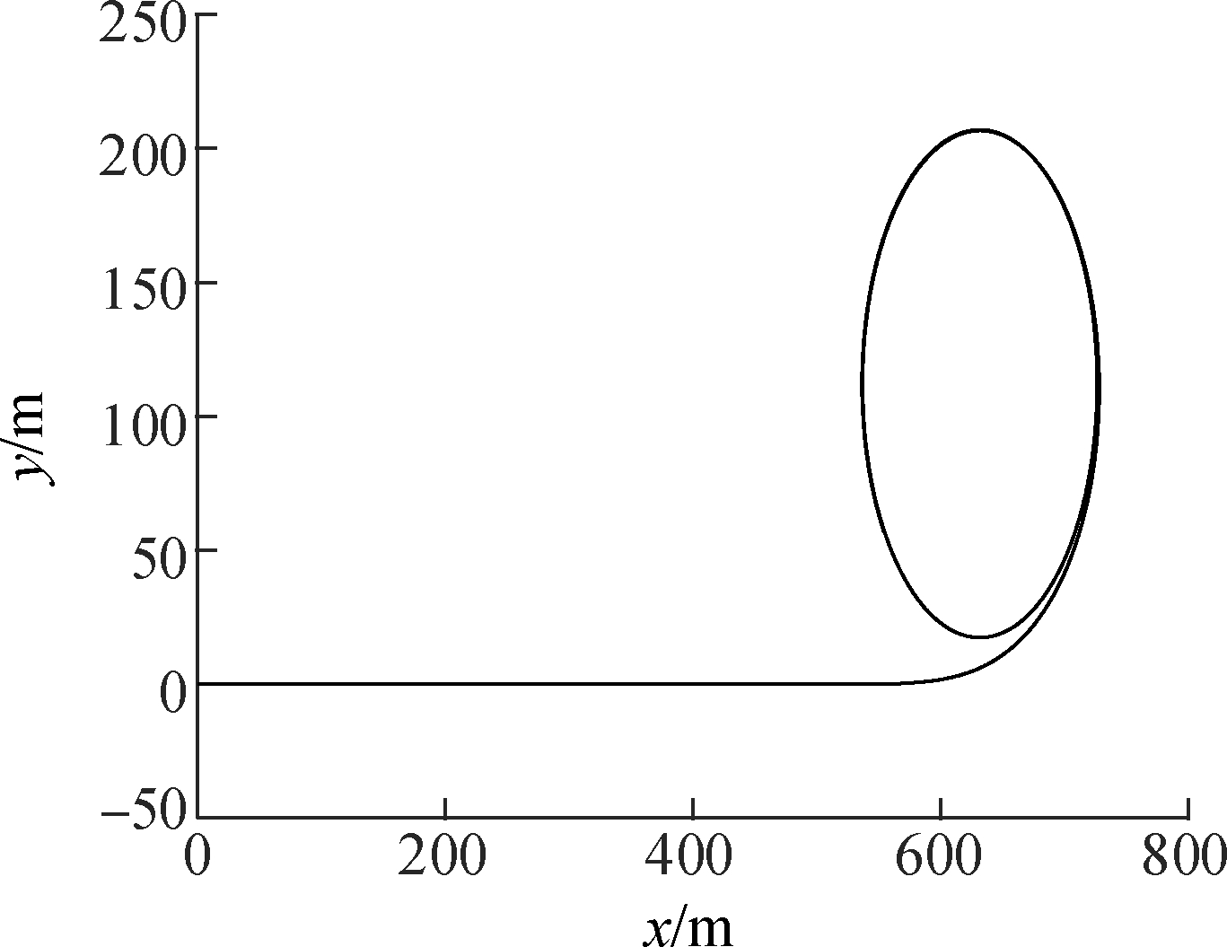
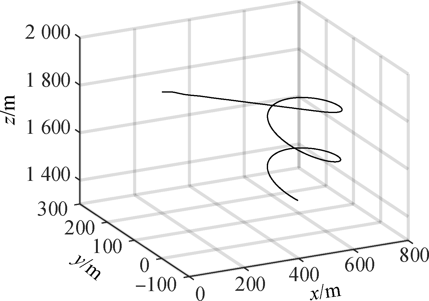
Fig.4 Simulation results of glide. (a) Trajectory in the horizontal plane; (b) Trajectory in 3D space; (c)Velocities and gliding ratio; (d) Euler angles
It can be seen that the vehicle glides steadily with the velocity in the x direction (vx) of 13.9 m/s, the velocity in the z direction (vz) of 4.5 m/s and the pitch angle of 6.9°. There are no yaw or roll motion in the gliding progress, and thus, the velocity in the y direction (vy) is 0, and the forward velocity (vF) and the resultant velocity (vR) are also 0. The gliding ratio (f) of the parafoil system stabilizes at 3, and the trajectories both in the horizontal plane and 3D space are straight lines.
3.1.2 Turning under unilateral deflection
The parafoil system turns under the condition of unilateral deflection. The working condition is set as follows: After 37.5 s, the left steering line is pulled down by 20%, and the corresponding flap deflection angle is 7°. With the deflection of the left flap on the left side of the parafoil canopy, the lift and drag forces increase, as does the resultant velocity of the parafoil system. Meanwhile, the vehicle begins to produce roll and yaw motion trends, and the pitch angle decreases to maintain the equilibrium of forces. For the whole system, the lift and drag forces lose, and the speed of the system eventually increases.
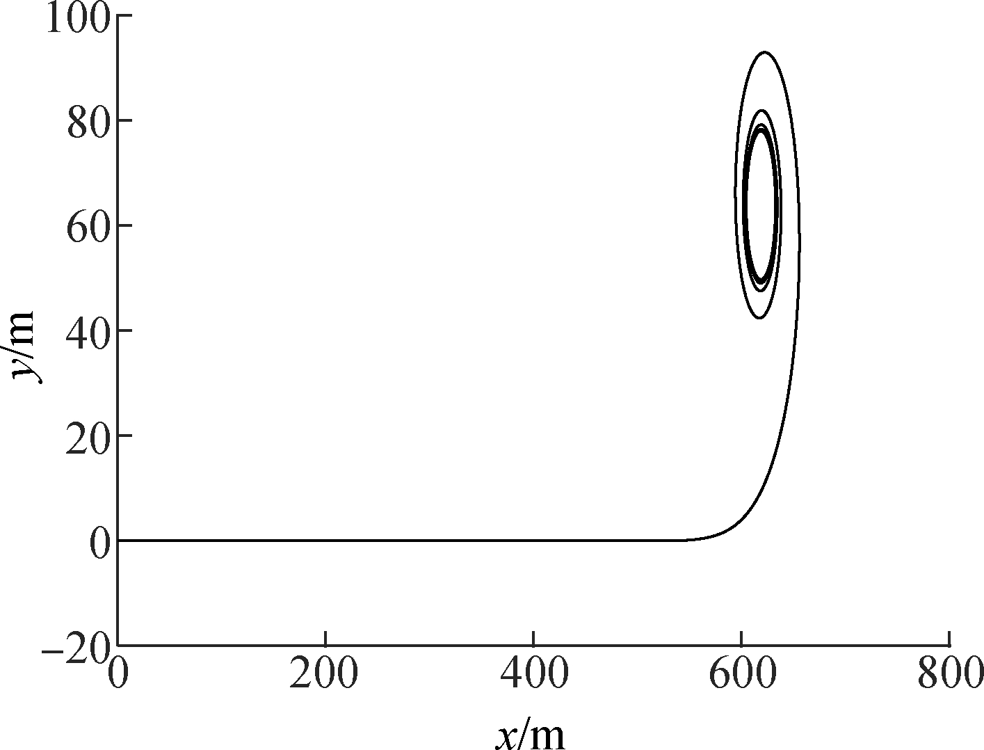
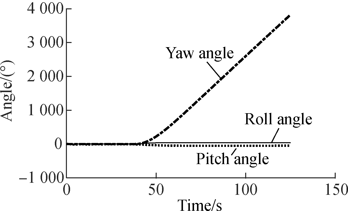
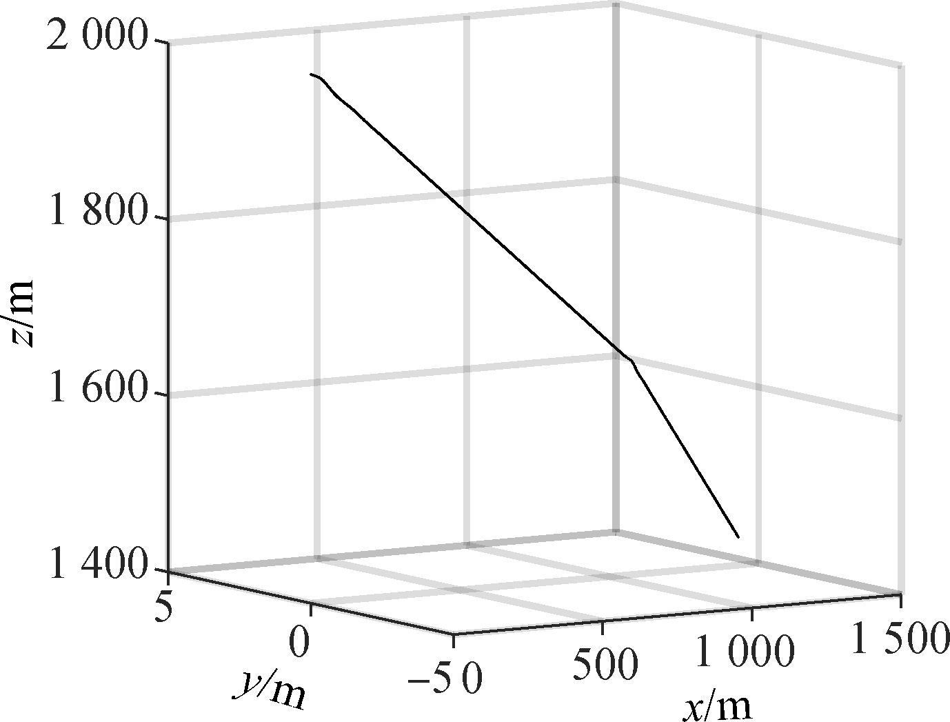
For analysis of motion characteristics, the velocities, gliding ratio, horizontal trajectory, 3D trajectory and Euler angles of the parafoil system are drawn in Fig.5.
It can be seen from Fig.5 that with unilateral deflection 20%, the horizontal trajectory is a circle with radius 94.8 m and the 3D trajectory is a downward spiral. Velocities vx and vy show a sine wave with a period of 156 s. The vertical velocity almost remains unchanged, and so do the forward velocity and resultant velocity. The gliding ratio stabilizes at 2.8. After deflecting, the vehicle shows a continuous yaw trend, while its pitch angle decreases from -8° to -10°, and its roll angle increases from 0 to 9°.
The magnitude of unilateral deflection is usually limited within a certain range, so as to avoid damaging the holistic stability of the system. Typically, when the unilateral deflection approaches 40%, the corresponding flap deflection angle is approximately 15°, the parafoil system will be in stall, in which the manipulation will worsen, and altitude will be lost quickly. As shown in Fig.6, velocity vz increases rapidly to 16.5 m/s, the roll angle increases to 37°, and the pitch angle reaches -49°. The parafoil canopy probably collapses and the vehicle will fall down within a very short time.
3.1.3 Flare landing
Flare landing, implemented in the final stages of landing, is realized by pulling down the left and right steering lines by 100% simultaneously and quickly, which can effectively reduce the velocity of landing and avoid the damage of payloads in the landing progress. The working condition is set as follows: After 37.5 s, when the vehicle is in the stable state of gliding, both steering lines are pulled down, and the corresponding flap deflection angle is 75°. The motion characteristics are shown in Fig.7.
(a)
(b)

(c)

(d)
Fig.5 Simulation results of turning. (a) Trajectory in the horizontal plane; (b) Trajectory in 3D space; (c) Velocities and gliding ratio; (d) Euler angles
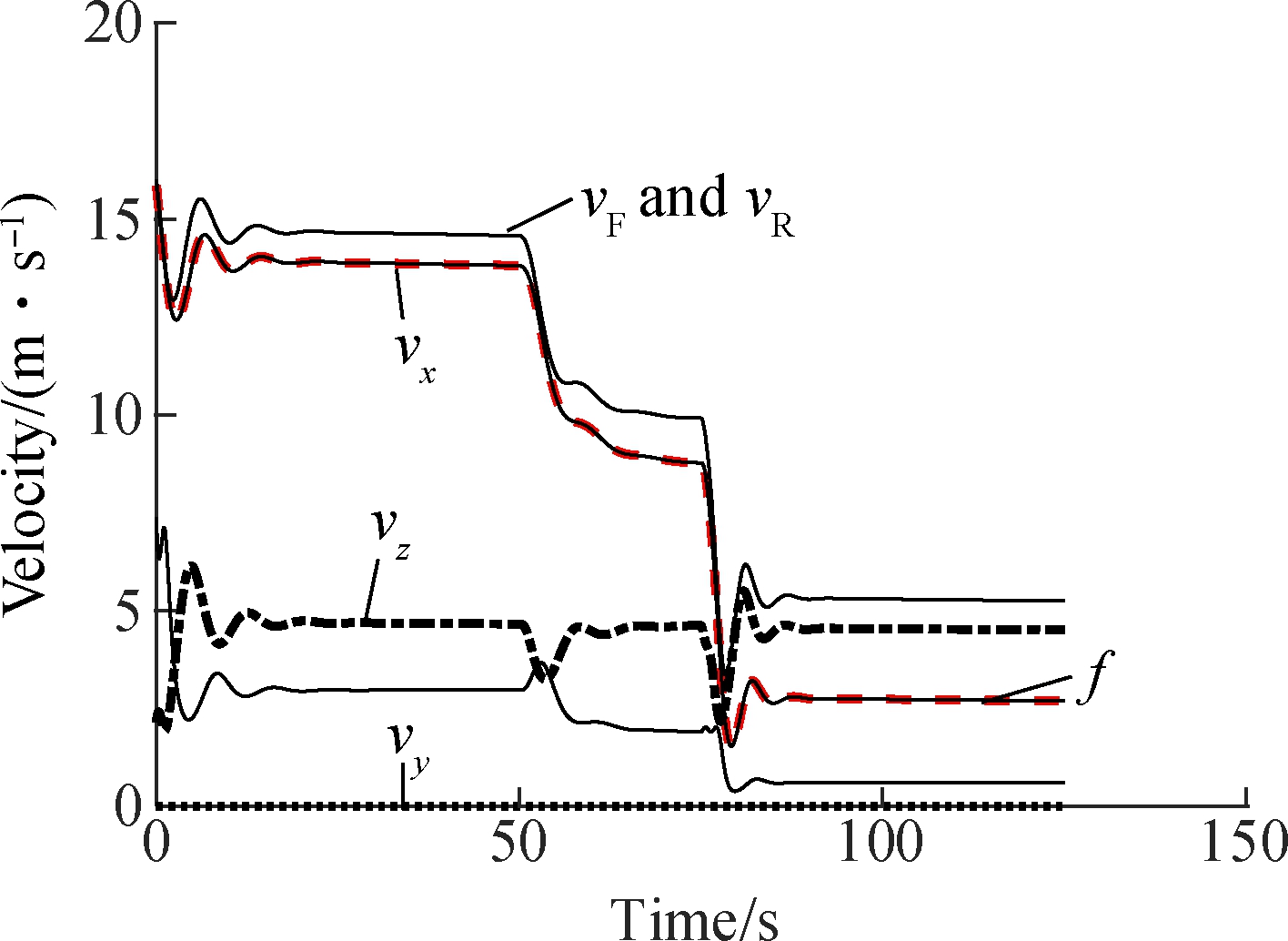
When deflecting the left and right flaps simultaneously, the lift and drag coefficients of both sides increase; however, the resultant velocity of the parafoil system decreases rapidly and soon reaches a new equilibrium state. At the same time, the system starts to show a pitch angle trend, with the pitch angel increasing from -7° to -12°, but with no roll or yaw motion.
It can be observed that when t=41.7 s, velocity vx decreases from 14.0 m/s to minimum 6.5 m/s; when t=40.2 s, velocity vz decreases from 5.0 m/s to minimum
(a)

(b)

(c)
(d)
Fig.6 Simulation results of stall condition. (a) Trajectory in the horizontal plane; (b) Trajectory in 3D space; (c) Velocities and gliding ratio; (d) Euler angles
2.0 m/s; after that, velocities vx and vz increase slightly, and finally the trend moves towards stabilization. The resultant velocity reaches minimum 7.5 m/s at 41.3 s. Velocity vx stabilizes at 7.8 m/s, and the resultant velocity stabilizes at 9 m/s, which is lower than before. Accordingly, bilateral deflection can realize the effects of deceleration, and if the time is chosen appropriately, the vehicle will land softly, just as the resultant velocity reaches the minimum.

(a)
(b)

(c)
(d)
Fig.7 Simulation results of flare landing. (a) Trajectory in the horizontal plane; (b) Trajectory in 3D space; (c) Velocities and gliding ratio; (d) Euler angles
Considering the fact that the parafoil system flying at a low altitude is more susceptible to winds, the influences of the transverse constant wind on gliding, turning and flare landing are discussed below.
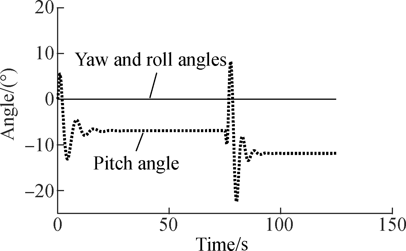
3.2.1 Gliding with winds
The working condition is set as follows: After 50 s, when the system is in the stable state of gliding, the transverse constant wind with a speed of 5 m/s and direction along the y axis is added into the simulation environment. The results are shown in Fig.8.
(a)

(b)

(c)
(d)
Fig.8 Simulation results of gliding with winds. (a) Trajectory in the horizontal plane; (b) Trajectory in 3D space; (c) Velocities and gliding ratio; (d) Euler angles
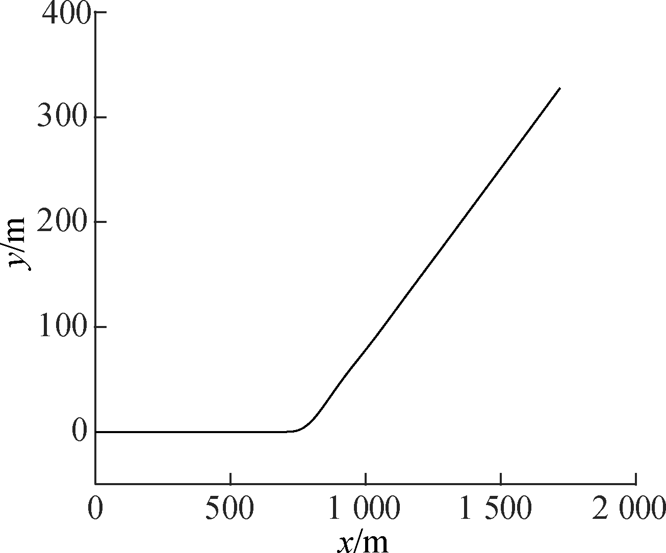
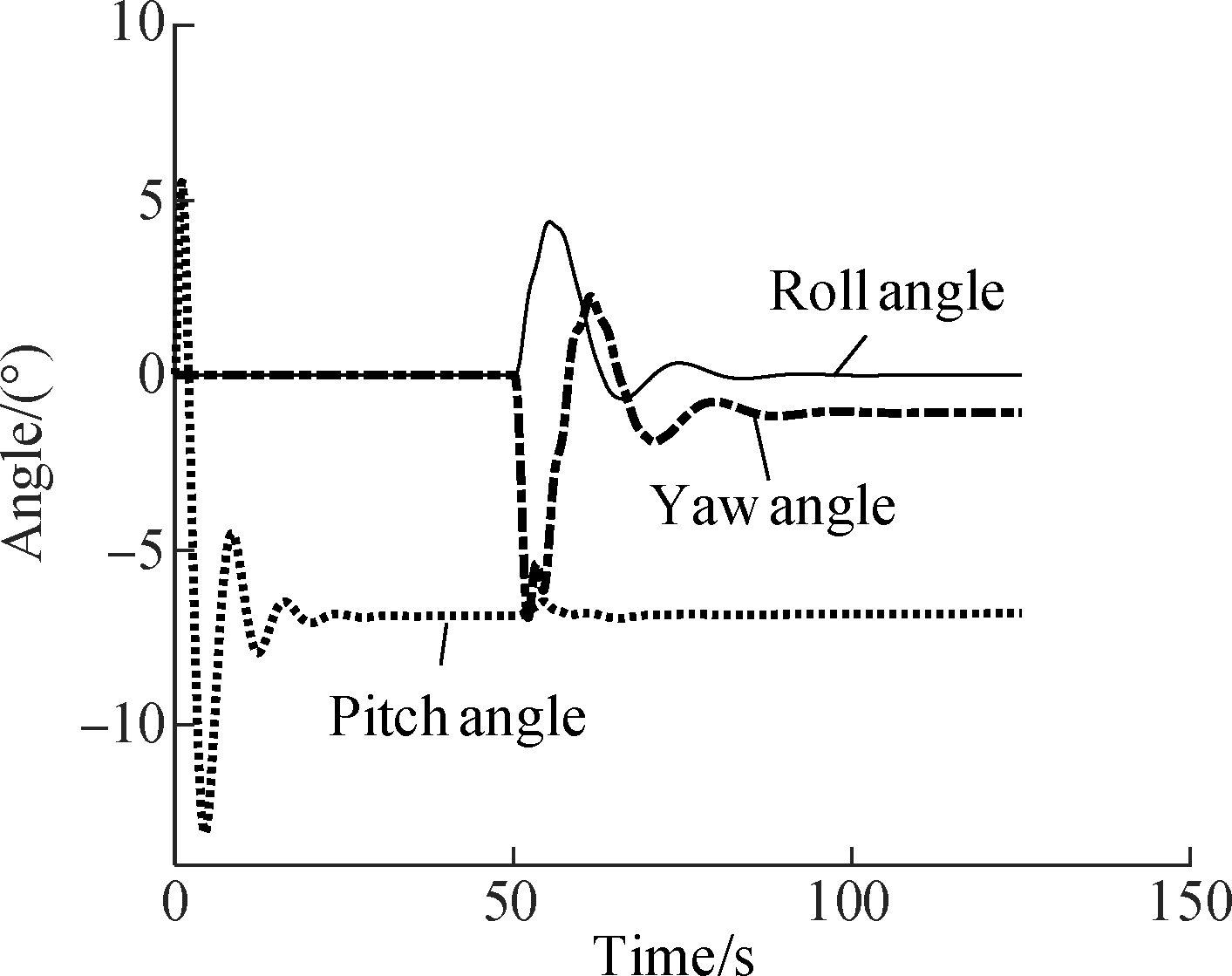
It can be seen from Fig.8 that influenced by the wind, the horizontal trajectory is an inclined straight line, and its slope is a constant value and corresponding to its yaw angle. Velocities vx and vz remain unchanged, while the ultimate y velocity is close to the wind speed, increasing from 0 to 4.6 m/s. Thus, the resultant velocity increases from 14.8 to 15.4 m/s, but the gliding ratio stays almost unchanged. At the start time of the wind, there are large fluctuations in the roll and yaw angles, but small changes in pitch angles. After being stabilized, a steady yaw trend is produced, and the yaw angle is less than 1.5°. It can be seen that the parafoil system will drift with the wind, and the velocity and direction of drifting depends on that of the wind.
3.2.2 Turning with winds
The working condition is set as follows: After 37.5 s, the left steering rope is pulled down by 20%, and then, after 50 s, when the vehicle is in the stable gliding state, the transverse constant wind with a speed of 5 m/s and direction along y axis is added into the simulation environment. The results are shown in Fig.9.
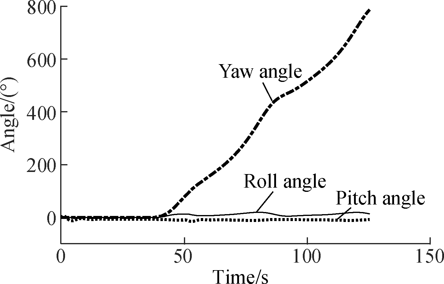
As shown in Fig.9, due to the influence of the wind, the horizontal trajectory is an upward spiral curve. Velocities vx and vy significantly fluctuate as a sine function curve. The z velocity sinusoidal fluctuates very slightly. The resultant velocity fluctuates from 11.3 to 20.5 m/s. The gliding ratio fluctuates from 1.7 to 3.6. From Fig.9(d), roll and yaw angles fluctuate slightly as a sine function curve, and a continuous yaw trend is produced.
3.2.3 Flare landing with winds
The working conditions are set as follows: After 50 s, the transverse constant winds with a speed of 5 m/s and direction along x axis and negative x axis are added into the simulation environment, respectively. After 75 s, as the system gliding steadily in the wind field, both steering lines are pulled down by 100% simultaneously and quickly. The simulation results are shown in Fig.10.
We can see that if the direction of wind is along the x axis, namely, the parafoil system flies against the wind, the resultant velocity decreases to 1.5 m/s after implementing flare landing; on the contrary, the resultant velocity only decreases to 11.3 m/s. Compared with the simulation results in Fig.7, it is clear that in the condition of upwind flare landing, the minimum velocity will be more close to zero; whereas flare landing follows the wind, the minimum velocity will be much larger. This may further explain that flying against the wind is a necessary condition for flare landing.
The airdrop test is a meaningful and convincing way to validate the dynamic model of parafoil systems. Our group have developed a small guided airdrop system, the specified parameters of which are the same as listed in Tab.1. To conduct the airdrop test, the parafoil system was lifted up and released through a hot air balloon. The basic information of the airdrop test is shown as follows: The elevation of the airdrop ground is 90 m, the elevation of the releasing site is 403 m, and the altitude loss of the

(a)

(b)

(c)
(d)
Fig.9 Simulation results of turning with winds. (a) Trajectory in the horizontal plane; (b)Trajectory in 3D space; (c) Velocities and gliding ratio; (d) Euler angles
parachute-opening is 40 m. The working condition is set as follows: The left steering line is pulled down by 50%. Thus, the data collection height interval is 273 m and the flight time is 105 s.
Location data collected by GPS module is in the form of latitude and longitude, and after conversion and processing, the results of the airdrop test are shown as the solid lines in Figs.11 and 12. As can be seen from the horizontal trajectory, the parafoil system is affected by the wind during the flight, and the wind direction and speed
(a)

(b)
Fig.10 The variation of velocities. (a) x axis wind; (b) negative x axis wind
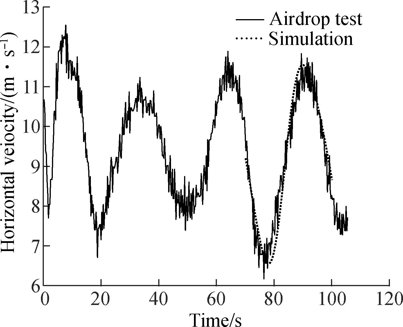
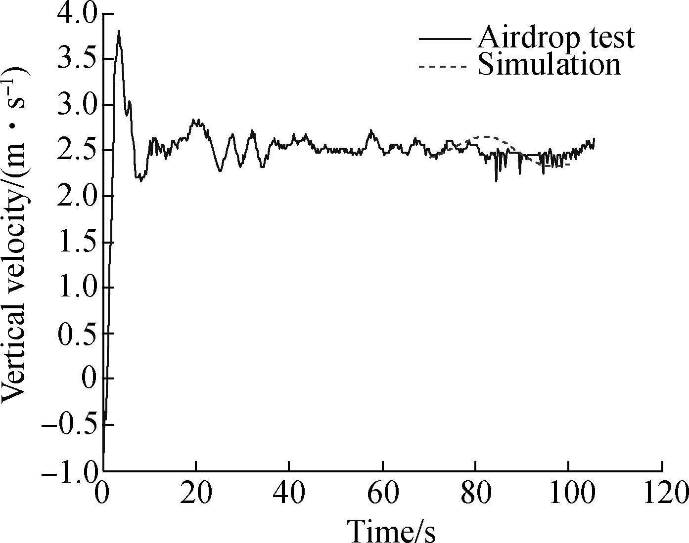
vary with height. In order to achieve better cognition of the landing area’s wind, we used LSM to estimate wind speed and direction according to GPS positioning data, and the details can be seen in Ref.[19]. On the basis of wind identification results, we intercepted airdrop test data from 71 s to 100 s. During the time, the vehicle is within 100 m from the ground; while the wind speed stabilizes at that of 2 m/s, and the wind direction remains stable at 160°. The parameters of the simulation model are set the same as that of the actual parafoil system of the airdrop test, and a similar wind is added into the simulated environment. Simulation data during the same time period is intercepted to compare with the airdrop test data, and the results are shown as the dotted lines in Figs.11 and 12.
From the comparative results in Fig.11, the simulation horizontal trajectory roughly overlaps with the flight track of the actual parafoil system, and local errors derive from the wind identification error and turbulences in the airdrop environment. As shown in Fig.12, the horizontal velocity of the simulation model is in good accordance with the airdrop test, with a deviation less than 0.5 m/s, while the vertical velocity of the parafoil system model fluctuates slightly under the influence of the wind, and shows a similar trend to the vertical velocity of the actual system. Through the above analysis, the established model can well describe the characteristics of the actual parafoil system.

Fig.11 Trajectories in the horizontal plane
(a)
(b)
Fig.12 Changing curves of velocities. (a) Changing curves of horizontal velocity; (b) Changing curves of vertical velocity
1) Regarding the parafoil and the payload as a rigid connection, the six DOF nonlinear dynamic model of the parafoil system including three DOF of translational motion with the mass center and the other three DOF of rotational motion around the mass center, was given according to the Kirchhoff motion equation.
2) Considering flap deflection as the control mechanism, the modeling process of which was relatively simple. The basic motion characteristics of glide, turn flare landing and their responses to transverse constant wind were analyzed through simulations.
3) Airdrop experiments were conducted to verify the model. The results show that the established model can accurately characterize the dynamic performance of the parafoil systems in windy conditions, which is of high value in engineering applications.
However, this model still needs further improvement. The relative motion between the parafoil and the payload, the control mode of flap defection, and more realistic wind field model should be considered and solved in the future research.
References
[1]Tao J, Sun Q L, Tan P L, et al. Active disturbance rejection control (ADRC)-based autonomous homing control of powered parafoils[J]. Nonlinear Dynamics, 2016, 86(3): 1461-1476. DOI:10.1007/s11071-016-2972-1.
[2]Yakimenko O A. Precision aerial delivery systems: Modeling, dynamics, and control [M]. Reston, USA: American Institute of Aeronautics and Astronautics, 2015: 263-265.
[3]Rogers J, Slegers N. Robust parafoil terminal guidance using massively parallel processing[J]. Journal of Guidance, Control, and Dynamics, 2013, 36(5): 1336-1345. DOI:10.2514/1.59782.
[4]Goodrick T F. Simulation studies of the flight dynamics of gliding parachute systems [C]//6th Aerodynamic Decelerator and Balloon Technology Conference. Houston, USA, 1979: 11-16. DOI:10.2514/6.1979-417.
[5]Iacomini C S, Cerimele C J. Lateral-directional aerodynamics from a large scale parafoil test program[C]//15th Aerodynamic Decelerator Systems Technology Conference. Toulouse, France, 1999: 218-228. DOI:10.2514/6.1999-1731.
[6]Zhang L M, Gao H T, Chen Z Q, et al. Multi-objective global optimal parafoil homing trajectory optimization via Gauss pseudospectral method [J]. Nonlinear Dynamics, 2013, 72(1): 1-8. DOI:10.1007/s11071-012-0586-9.
[7]Tao J, Sun Q L, Zhu E L, et al. Homing trajectory planning of parafoil system based on quantum genetic algorithm[J]. Journal of Harbin Engineering University, 2016, 37(9): 1261-1268.
[8]Barrows T M. Apparent mass of parafoils with spanwise camber [J]. Journal of Aircraft, 2002, 39(3): 445-451. DOI:10.2514/2.2949.
[9]Xiong J. Research on the dynamics and homing project of parafoil system [D]. Changsha: College of Aerospace and Materials Engineering, National University of Defense Technology, 2005. (in Chinese)
[10]Jiao L, Sun Q L, Kang X F, et al. Autonomous homing of parafoil and payload system based on ADRC [J]. Control Engineering and Application Informatics, 2011,13(3): 25-31.
[11]Slegers N. Effects of canopy-payload relative motion on control of autonomous parafoils [J]. Journal of Guidance Control and Dynamics, 2010, 33(1): 116-125. DOI:10.2514/1.44564.
[12]Ochi Y, Watanabe M. Modelling and simulation of the dynamics of a powered paraglider[J]. Proceedings of the Institution of Mechanical Engineers, Part G: Journal of Aerospace Engineering, 2011, 225(4): 373-386. DOI:10.1177/09544100jaero888.
[13]Yakimenko O A, Slegers N J. Using direct methods for terminal guidance of autonomous aerial delivery systems[C]//2009 European Control Conference. Budapest, Hungary, 2009: 2372-2377.
[14]Zhu E L, Sun Q L, Tan P L, et al. Modeling of powered parafoil based on Kirchhoff motion equation [J]. Nonlinear Dynamics, 2015, 79(1): 617-629. DOI:10.1007/s11071-014-1690-9.
[15]Tao J, Sun Q L, Tan P L, et al. Autonomous homing control of a powered parafoil with insufficient altitude[J]. ISA Transactions, 2016, 65: 516-524. DOI:10.1016/j.isatra.2016.08.016.
[16]Prakash O, Ananthkrishnan N. Modeling and simulation of 9-DOF parafoil-payload system flight dynamics [C]//AIAA Atmospheric Flight Mechanics Conference and Exhibit. Keystone, USA, 2006: 21-24.
[17]Yu G. Nine-degree of freedom modeling and flight dynamic analysis of parafoil aerial delivery system[C]//2014 Asia-Pacific International Symposium on Aerospace Technology. Shanghai, China, 2014: 866-872. DOI:10.1016/j.proeng.2014.12.614.
[18]Wang L R. Parachute theory and application[M]. Beijing: Aerospace Press, 1997: 158-161. (in Chinese)
[19]Tan P L, Sun Q L, Gao H T, et al. Wind identification and application of the powered parafoil system[J]. Acta Aeronautica et Astronautica Sinica, 2016, 37(7):2286-2294. DOI:10.7527/S1000-6893.2016.0091. (in Chinese)
摘要:为更好地研究翼伞系统的动力学特性和控制策略,将襟翼偏转作为翼伞控制机制,伞体和回收物视为刚性连接,根据克西霍夫运动方程建立了翼伞系统六自由度模型,包括随质心的三自由度平动和绕质心的三自由度转动.由于翼伞系统由柔性结构的冲压型翼伞提供升力,且飞行高度较低,容易受到环境中风场的影响,因此对有风和无风环境下翼伞系统的基本运动特性进行了仿真分析,并利用空投实验对所建立模型进一步验证.仿真和空投实验对比结果表明,翼伞系统仿真轨迹和空投实际轨迹基本上能够吻合,其水平仿真速度与空投实验误差小于0.5 m/s,垂直仿真速度在风场作用下呈现小幅波动,与空投实验结果一致,说明该模型能够有效地描述翼伞系统的运动性能.
关键词:翼伞系统; 动态建模与仿真; 飞行特性; 空投实验; 襟翼偏转
中图分类号:V19
DOI:10.3969/j.issn.1003-7985.2017.04.005
Received 2017-04-10,
Revised 2017-08-12.
Biographies:Tao Jin (1986—), male, doctor; Sun Qinglin (corresponding author), male, doctor, professor, sunql@nankai.edu.cn.
Foundation items:The National Natural Science Foundation of China (No.61273138, 61573197), the National Key Technology R & D Program (No.2015BAK06B04), the Key Fund of Tianjin (No.14JCZDJC39300), the Key Technologies R & D Program of Tianjin (No.14ZCZDSF00022).
Citation:Tao Jin, Sun Qinglin, Chen Zengqiang, et al. Dynamic modeling of a parafoil system considering flap deflection[J].Journal of Southeast University (English Edition),2017,33(4):416-425.
DOI:10.3969/j.issn.1003-7985.2017.04.005.