Abstract:Aiming at the problem of the low accuracy of low dynamic vehicle velocity under the environment of uneven distribution of light intensity, an improved adaptive Kalman filter method for the velocity error estimate by the fusion of optical flow tracking and scale invariant feature transform (SIFT) is proposed. The algorithm introduces a nonlinear fuzzy membership function and the filter residual for the noise covariance matrix in the adaptive adjustment process. In the process of calculating the velocity of the vehicle, the tracking and matching of the inter-frame displacement and the vehicle velocity calculation are carried out by using the optical flow tracing and the SIFT methods, respectively. Meanwhile, the velocity difference between the outputs of these two methods is used as the observation of the improved adaptive Kalman filter. Finally, the velocity calculated by the optical flow method is corrected by using the velocity error estimate of the output of the modified adaptive Kalman filter. The results of semi-physical experiments show that the maximum velocity error of the fusion algorithm is decreased by 29% than that of the optical flow method, and the computation time is reduced by 80% compared with the SIFT method.
Key words:velocity; optical flow; feature point matching; non-uniform light intensity distribution
Traditionally, the task of computing speed is usually performed using imprecise wheel speed sensors and inertial measurement units[1] or expensive high accuracy inertial measurement units[2]. In recent years, it has become an important requirement to obtain the speed of the vehicle based on vision. In comparison with wheel odometry, the visual method is not affected by wheel slippage in slippery or uneven terrain or other abnormal conditions, which can provide more accurate speed estimates[3]. The visual method is useful for various reasons due to the fact that cameras are fairly small and inexpensive, and they can obtain a greater data stream of the surrounding environment, by which the speed of the robot or vehicle can be accurately estimated[4].
In a uniform light intensity distribution environment, the visual method of obtaining velocity has high precision and is an excellent complement to wheel odometry or other navigation systems such as the global positioning system or inertial measurement units[5]. In Ref.[6], the BRISK and SURF feature point matching algorithms are used to measure the vehicle speed, which can ensure the robustness in the uneven distribution of light intensity, but the real-time performance is poor. Kitt et al.[7] proposed a robust optical flow method for accurately estimating the attitude of UAV, which is fast and the image motion estimation meets the requirements of high precision and stability, nevertheless the accuracy of the motion velocity estimated by this method is markedly influenced by illumination.
In this paper, a new method is proposed to calculate the velocity of a low dynamic vehicle, which is based on the fusion of optical flow and feature matching under the condition of uneven distribution of light intensity. By the vehicle driving test in a non-uniform intensity environment, the results show that this method overcomes the shortcomings of the optical flow and the SIFT feature matching methods while the estimation accuracy and real-time performance are improved significantly.
The Lucas-Kanade optical flow algorithm proposed by Lucas et al.[8] has been widely used for optical flow estimation, which is used to obtain the optical flow value by assuming that the optical flow in the local neighborhood of the pixel of interest is invariant and then solving the elementary optical flow equation constructed by all the pixels around the neighborhood of the pixel of interest by the least square method. Bouguet[9] proposed a Lucas-Kanade algorithm based on pyramid layering to cope with the problem of using the Lucas-Kanade algorithm, which means that the condition that the inter-frame displacement should be small enough must be satisfied. This algorithm is summarized in the following.
For a point u(ux,uy) in the current frame image Ik-1, a point v(ux+dx,uy+dy) is found in the next frame image Ik, which has the most similar gray values to u(ux,uy) and the vector d=[dx,dy] represents the optical flow of the pixel u.
We define the gray value difference between the two consecutive frames as
ε(d,A)=ε(dx,dy,dxx,dxy,dyx,dyy)=
![]() (Ik-1(x+ux,y+uy)-Ik([x,y]AT+d+u))
(Ik-1(x+ux,y+uy)-Ik([x,y]AT+d+u))
(1)
where A=![]() is the transformation matrix, and dxx, dxy, dyx and dyy are the affine deformation parameters.
is the transformation matrix, and dxx, dxy, dyx and dyy are the affine deformation parameters.
This algorithm achieves the purpose of calculating the optical flow by finding vector d and transformation matrix A, so that the gray scale difference of the consecutive frames is minimum.
This algorithm also needs to build an image pyramid by down-sampling. First, the optical flow is calculated by the top-level image in the image pyramid, and then the optical flow is used to estimate the position of the corresponding pixel in the next layer pyramid. These processes are repeated until the image pyramid of the bottom is calculated. According to this method, the horizontal and vertical displacements of the feature points of the consecutive frames are tracked and matched. Subsequently, all the displacement is accumulated and averaged to obtain the pixel displacement [![]() ]T between the consecutive frames. The image pixel velocity [
]T between the consecutive frames. The image pixel velocity [![]() ]T can be calculated as
]T can be calculated as
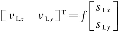
(2)
where f is the frequency of the camera.
In this paper, SIFT[10] is used to extract feature points for matching, so as to estimate the speed between two adjacent frames. First, the SIFT feature matching algorithm is used to establish the scale space, and the representation of an image in different scale space can be obtained by convolving the original image I with a set of variable-scaled Gaussian G:
L(x,y,σ)=G(x,y,σ)*I(x,y)
(3)
where L stands for the scale space and σ denotes the scale space factor.
In order to ensure that the extreme stable points are detected in both the scale space and two-dimensional image space, the DOG (difference-of-Gaussian) operator is applied to approximate the Laplacian-Gaussian operator. Suppose that the approximate operator is D(x,y,σ), after processing the image, we have
D(x,y,σ)=L(x,y,kσ)-L(x,y,σ)
(4)
where k is the constant factor.
After approximating the Laplacian-Gaussian operator by the DOG operator, extrema detection is required in DOG scale space. The gray scale value of the point to be detected is compared with 18 pixels at the corresponding position of the front and rear images in the scale space, as well as the surrounding ones of the point itself. Altogether, a single point requires 26 comparisons. When an extremum (maximum or minimum) is detected, it is kept for further processing.
Local extrema detected in DOG scale-space are called keypoints after the operations of improving positioning accuracy and eliminating low-contrast points. To locate the keypoints accurately, the principal curvature and keypoint orientation should be determined. The principal curvature calculated by the Hessian matrix and a threshold is used to remove the unstable edge response. The orientation is determined by the distribution characteristics of the gradient magnitude of the keypoints. The gradient magnitude m(x,y) and orientation θ(x,y) can be expressed as
m(x,y)= ((L(x+1,y)-L(x-1,y))2+
(L(x,y+1)-L(x,y-1))2)1/2
(5)
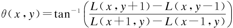
(6)
An orientation histogram is formed from the gradient orientations θ of sample points in the region around the keypoints, and the peak of the histogram as the main direction of the keypoint while the information of the key point is given and it is further descripted by generating the eigenvector descriptor.
After the descriptor is generated, the Euclidean distance of the feature vector is used as the feature point matching criterion, and the image velocity is calculated by the successful matched feature points.
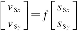
(7)
where sSx is the average horizontal displacement of feature points, and sSy is the vertical displacement.
In our experiments, the camera is mounted on the front of the vehicle and the optical axis is perpendicular to the ground surface to achieve the vertical photography of the ground texture[11-12]. The speed measurement model is shown in Fig.1. P(XR,YR,ZR) is a point on the ground which is projected onto the normalized image plane. ZR is the distance from the camera projection center to the ground, and R is the projection point of the optical center of the camera on the ground.
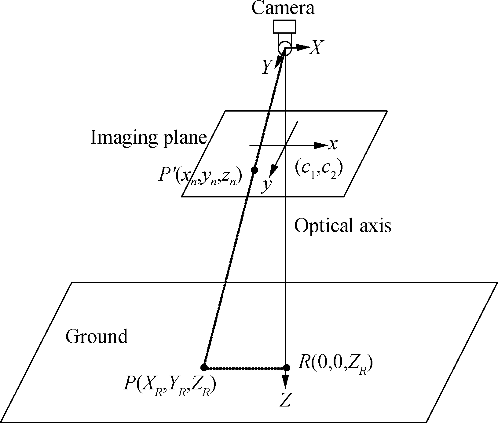
Fig.1 Speed measurement model
The relationship between the projection point P′(xn,yn,zn) and P(xR,yR,zR) can be expressed as

(8)
Taking the camera lens distortion effects into account, P′(xn,yn,zn) is the actual image point and P″(xd,yd,zd) is the ideal image point. The relationship of the distortion correction is
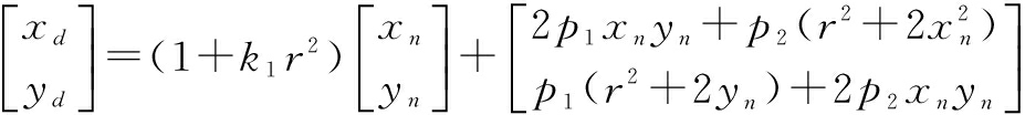
(9)
where r=![]() ; k1 is the coefficient of radial distortion; p1 and p2 denote the coefficients of axial distortion.
; k1 is the coefficient of radial distortion; p1 and p2 denote the coefficients of axial distortion.
In order to estimate the velocity of the vehicle, P″(xd,yd,zd) is mapped to the point P‴(xp,yp,zp) in the physical image coordinate system. The specific mapping relationship is
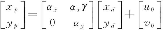
(10)
where αx and αy are the focal distances expressed in units of horizontal and vertical pixels; γ is the skewness coefficient; and (u0,v0) denotes the principal point coordinate of the image plane.
In order to simplify the calculation, we assume that there is no distortion effect in the camera lens, so k1, p1, p2 and γ are 0. Eq.(10) can be rewritten as

(11)
Differentiating time in Eq.(11), the velocity of the vehicle can be derived from the x and y axes of the world coordinate system:

(12)
where vx and vy represent the pixel speed of the images. It is assumed that the terrain surface is flat during the movement of the vehicle, so VZ=0 and Eq. (12) can be simplified as
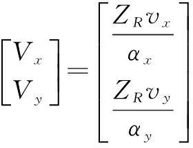
(13)
The vehicle velocity ![]() solved by the optical flow method can be obtained from Eqs.(2) and (13), and the velocity
solved by the optical flow method can be obtained from Eqs.(2) and (13), and the velocity ![]() solved by feature matching can be obtained by Eqs.(7) and (13).
solved by feature matching can be obtained by Eqs.(7) and (13).
In this paper, an improved adaptive Kalman filter is proposed to fuse the optical flow and the feature matching to calculate the velocity of the vehicle so as to overcome the problems of the low precision of the pyramid Lucas-Kanade optical flow and time-consuming of the SIFT feature matching. Fig.2 illustrates the fusion algorithm using a block diagram.
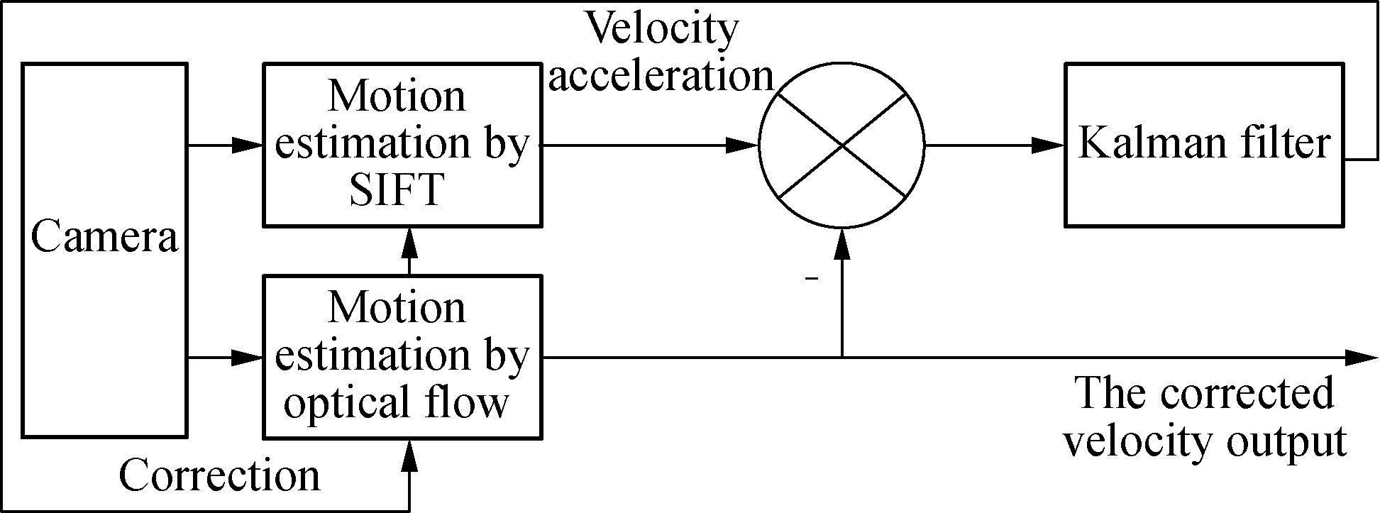
Fig.2 The structure diagram of the fusion algorithm
In the case when the vehicle only moves forward, the velocity in the traveling direction of the vehicle can be expressed by VLy and VSy. The acceleration difference Va and the speed difference ΔV* are the state variables which are solved by the improved adaptive Kalman filter. The difference ΔV between VLy and VSy obtained by visual measurement at each moment is regarded as a measurement.
In general, the calculation speed of the optical flow is faster than that of the SIFT in calculating the visual velocity information. In order to realize the synchronization of speed, the displacement between two consecutive frames is calculated and accumulated by the optical flow method. The average vehicle speed is obtained every 10 frames, and the first and tenth frames are matched by using SIFT to obtain another vehicle speed. Finally, the fusion of these two speeds is carried out.
The state model and measurement model of the filter are shown as follows:
X(k)=Φ(k|k-1)X(k-1)+U(k-1)Δ![]() +W(k-1)
+W(k-1)
(14)
Z(k)=H(k)X(k)+V(k)
(15)
where Φ(k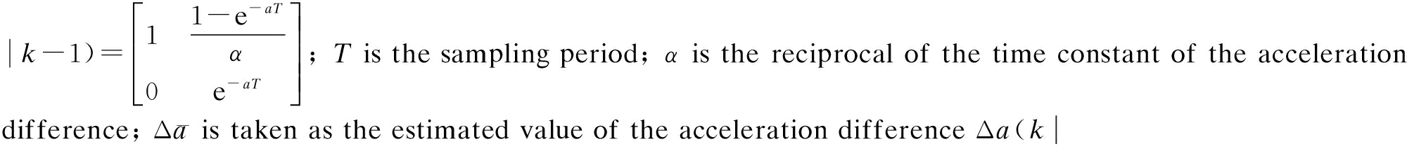 k-1) at time k;
 ![]() ; H(k)=
; H(k)=![]() ; V(k) stands for the noise of the measurement model.
; V(k) stands for the noise of the measurement model.
The covariance matrix Q(k-1) of the system noise is
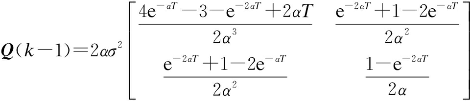
(16)
The adaptive implementation of the algorithm is based on the current acceleration difference Δa(k|k) and the filter residual error err(k) of the vehicle, which adjust the variance σ2 of the current acceleration difference, to fulfill the adaptive adjustment of Q(k-1). The variance σ2 of the acceleration difference is given by

(17)
where Δanew-max and Δanew-min are the maximum and the minimum value, which can be achieved after the adaptive adjustment of the acceleration difference. And, they change with the change of Δa(k|k).
Δa-up and Δaup are the limit values of the acceleration difference of the vehicle before adjustment, so the acceleration difference of the vehicle is within the interval [Δa-up,Δaup] and the two thresholds Δay and Δa-y are set such that Δay>Δaup and Δa-y<Δa-up, then the value of Δanew-max and Δanew-min are adjusted by the nonlinear fuzzy membership function of the exponential form. Δanew-max and Δanew-minare obtained by
(18)
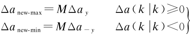
(19)
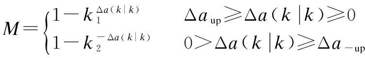
In order to further improve the estimation accuracy of the filtering algorithm, the filter residual error err(k) is introduced to adjust coefficients k1 and k2. k1 and k2 can be expressed as

(20)

(21)
err(k)=Z(k)-H(k)X(k|k-1)
(22)
where n is a positive number set according to human experience and only when ||err(k)![]() 0,
0,![]() 0,
0,![]() exp
exp![]() ,
,![]() .
.
Finally, the modified adaptive Kalman filter is used to directly correct the vehicle velocity solved by the optical flow, which can achieve higher precision vehicle speed.
Our velocity measurement system consists of a vehicle, a downward-looking camera, a PC, a DC motor and its built-in encoder (see Fig.3). In the experiment, we con-trol the vehicle running in the indoor light intensity distribution uneven environment with a downward-looking camera mounted on the front of the vehicle to acquire image sequences of a carpeted floor surface at a frame rate of 20 frame/s, and each frame image has a 320×240 pixels resolution. An encoder is provided on the wheel of the vehicle to collect the vehicle velocity VE, and the velocity information as a reference value is used to compare the corrected velocity. The speed of the vehicle is about 15 cm/s.
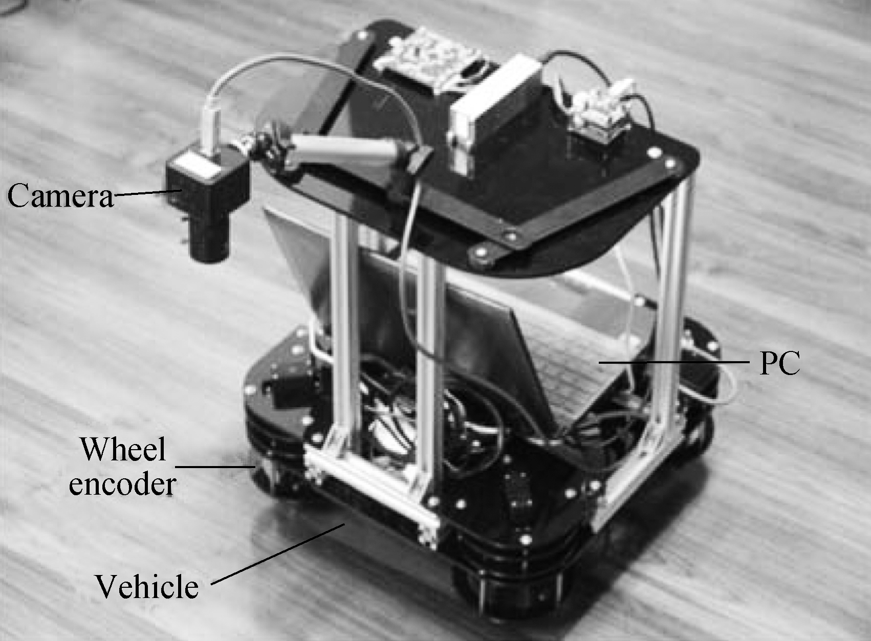
Fig.3 Velocity measurement system
We can see from Fig.4 that the speed of the SIFT measurement is less affected by the intensity of light than that measured by the optical flow. In Fig.5, TF and TS represent the time consumed by the optical flow and the SIFT, which illustrates that the real-time performance of the optical flow is better than that of the SIFT. As shown in Fig.6, after using the fusion algorithm of optical flow and feature matching, the corrected vehicle velocity VCL is less affected by the light intensity and it tends to the true value of the speed of the vehicle. Fig.7 presents that the error curve eCL of the corrected speed has a smaller fluctuation than that previous correction and eCLtends to zero. In brief, we can obtain a higher accuracy of the vehicle speed based on the combination of optical flow and feature point matching.
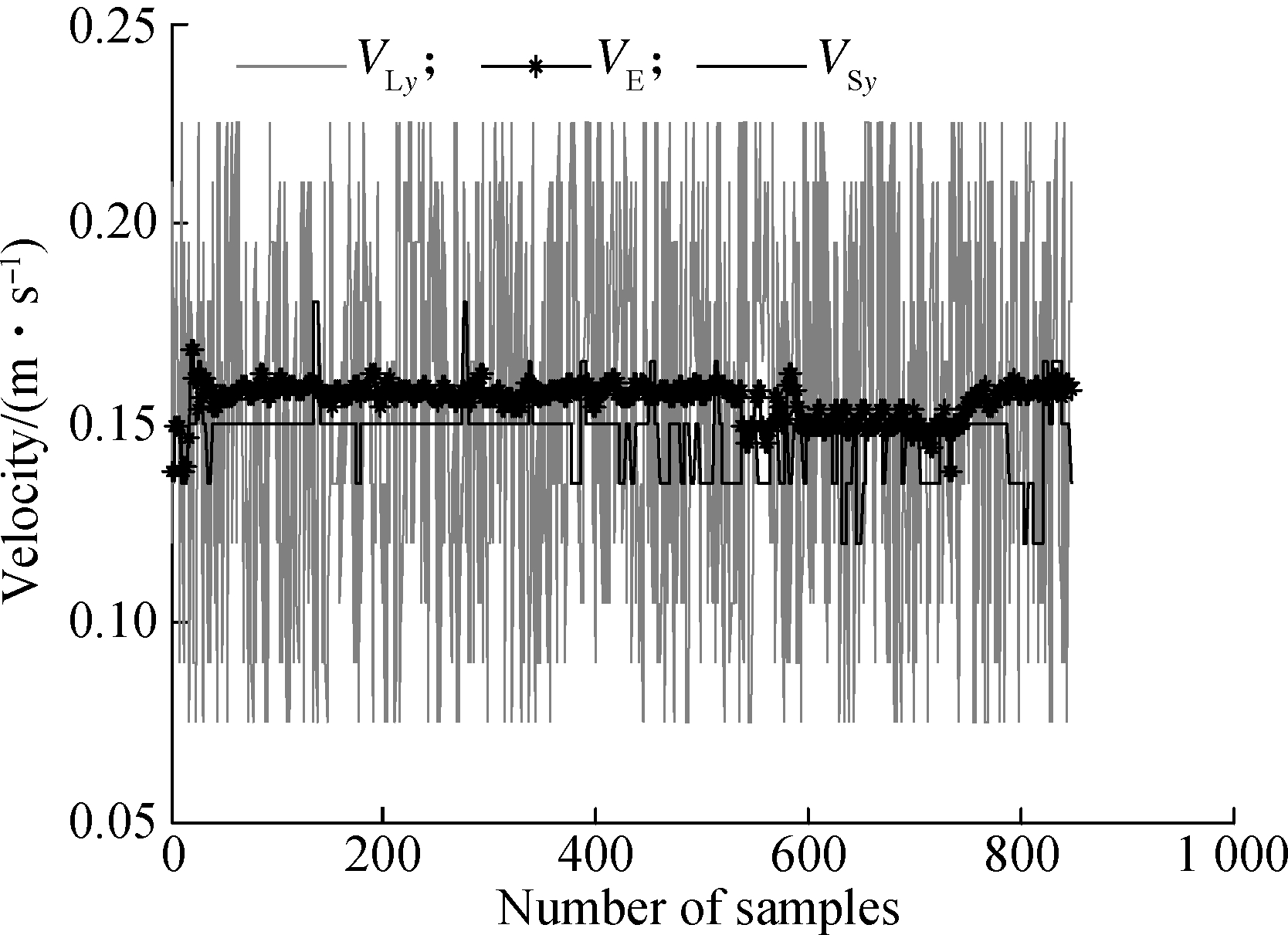
Fig.4 Comparison of the velocity measured by optical flow, SIFT and encoder
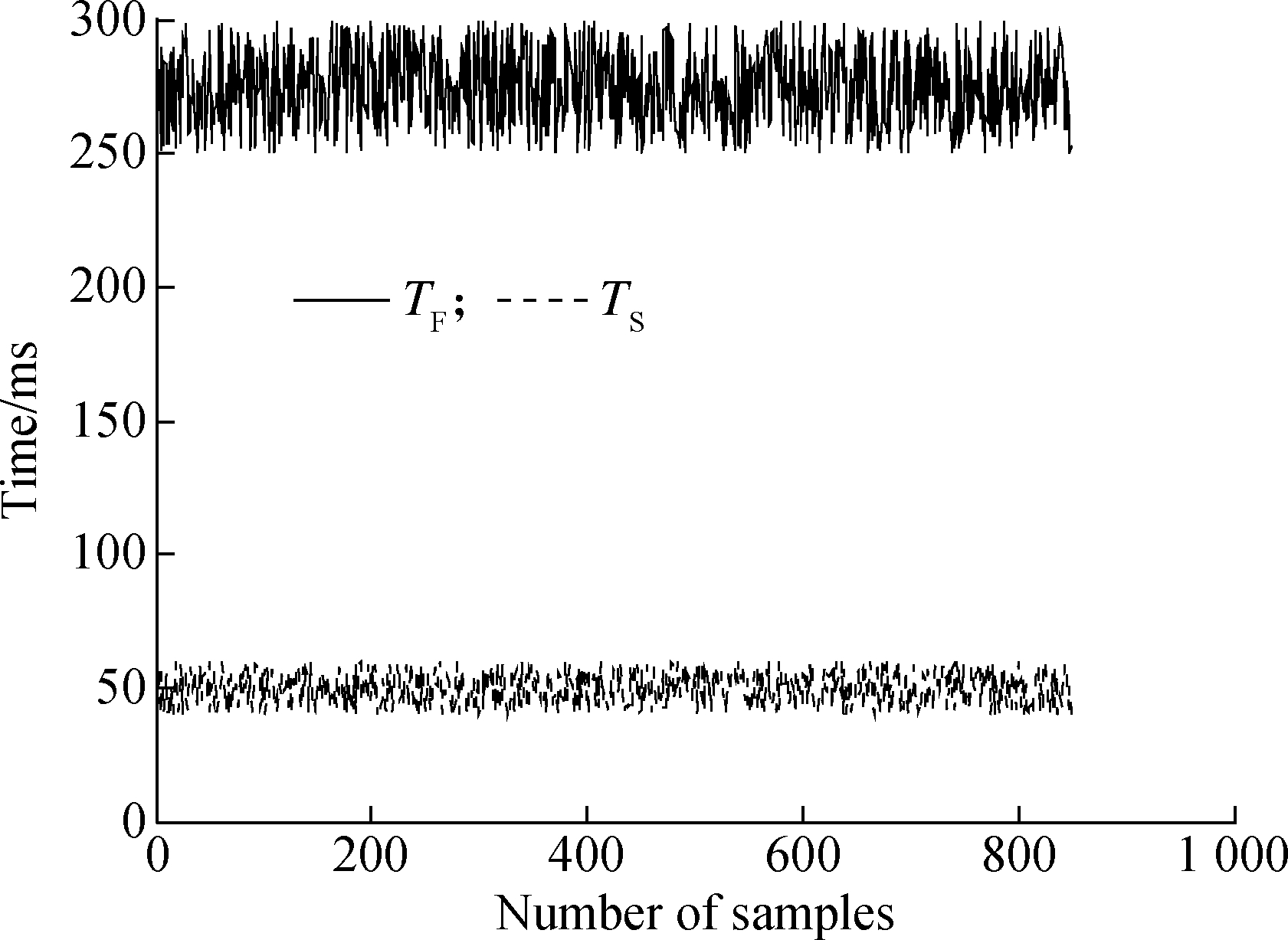
Fig.5 Comparison of processing time
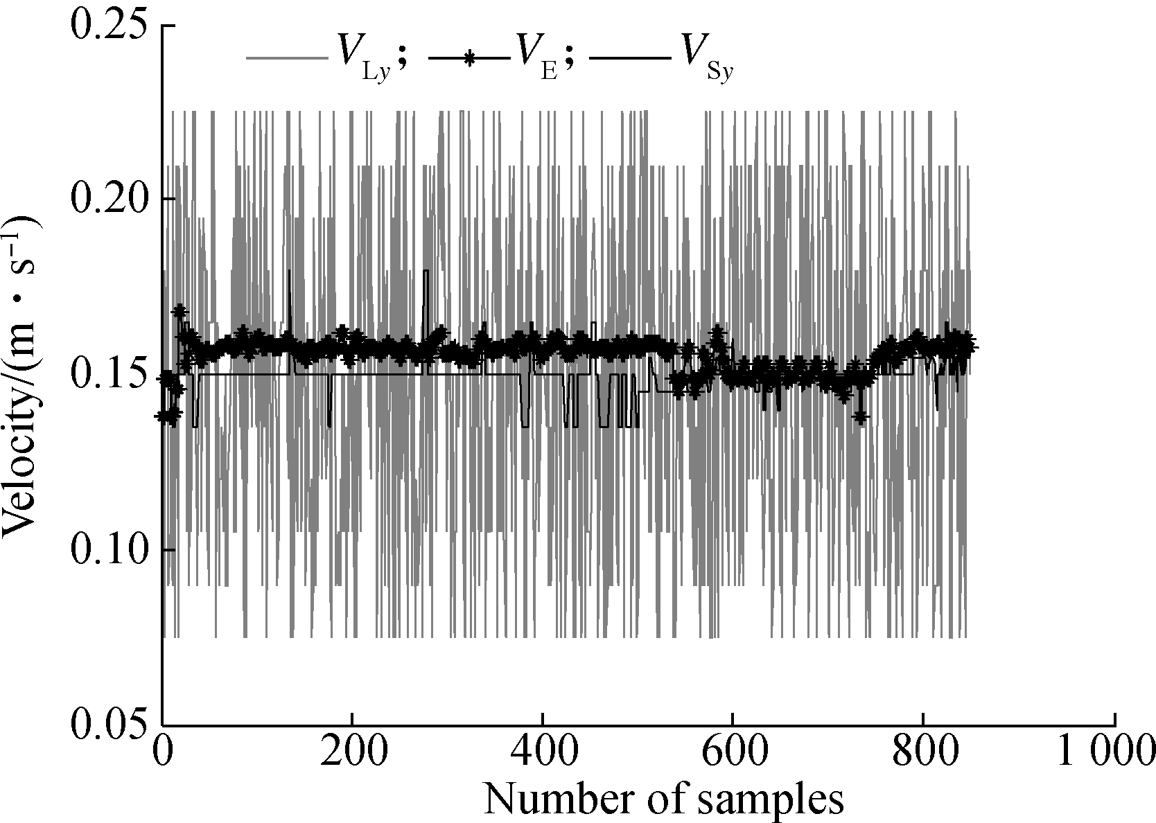
Fig.6 Velocity measured by the encoder and the optical flow before and after the correction
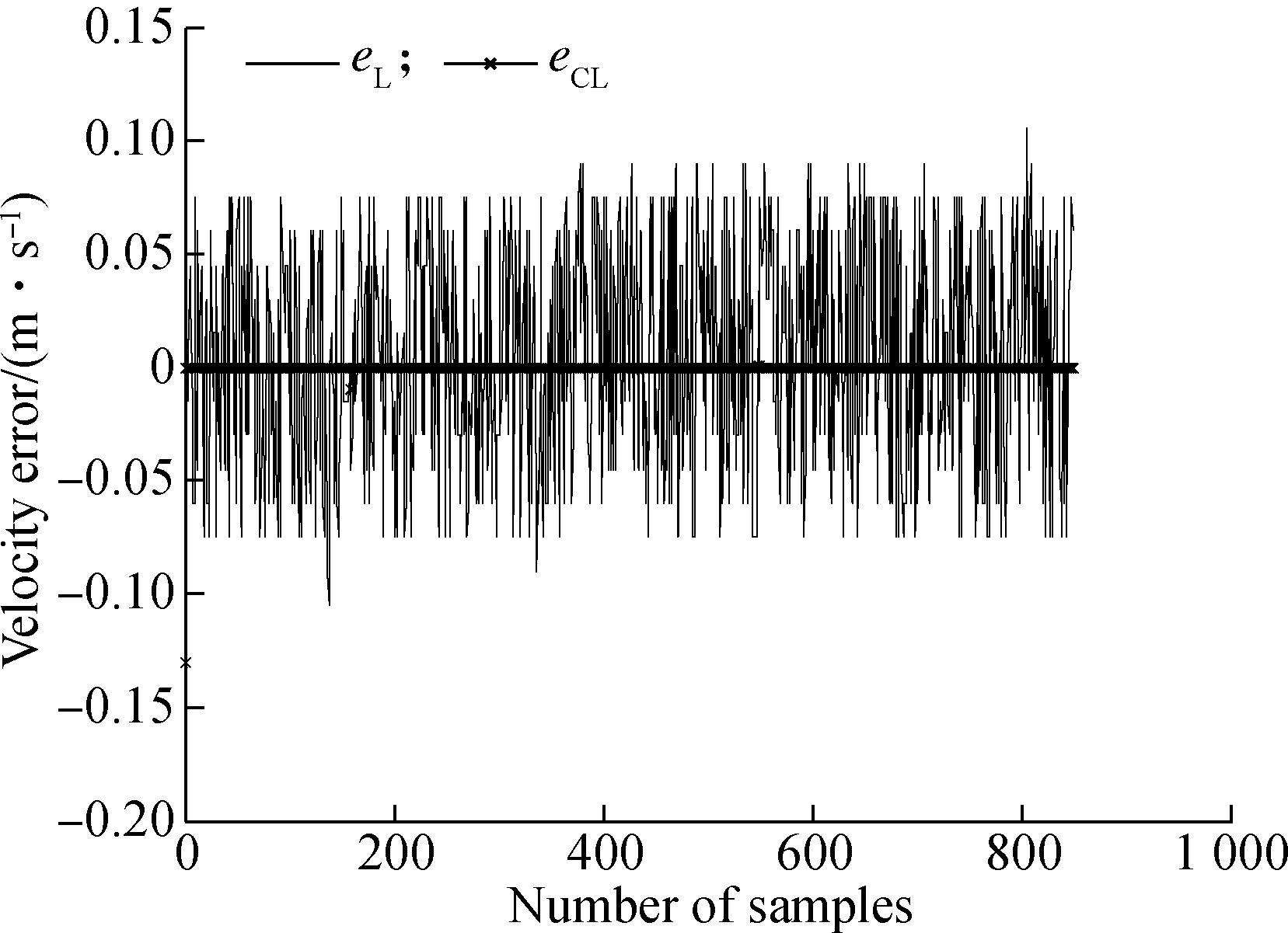
Fig.7 Velocity error before and after correction
In this paper, we present an improved adaptive Kalman filter to fuse the optical flow tracking method with the SIFT feature matching to solve the problem of the low accuracy of the low dynamic vehicle velocity calculation under the non-uniform light intensity distribution. The experimental results show that the fusion algorithm not only highlights the real-time characteristics of optical flow and the accuracy of SIFT feature matching, but also improves the estimation accuracy and real-time performance of low dynamic vehicle velocity under non-uniform light intensity distribution. The algorithm is instructive to visually aid navigation.
References
[1]Howard A. Real-time stereo visual odometry for autonomous ground vehicles[C]//IEEE/RSJ International Conference on Intelligent Robots and Systems. Nice, France, 2008: 3946-3952.DOI: 10.1109/IROS.2008.4651147.
[2]Kitt B, Geiger A, Lategahn H. Visual odometry based on stereo image sequences with RANSAC-based outlier rejection scheme[C]//2010 IEEE Intelligent Vehicles Symposium. San Diego, CA, USA, 2010: 486-492. DOI: 10.1109/IVS.2010.5548123.
[3]Scaramuzza D, Fraundorfer F. Visual odometry: Part Ⅰ: The first 30 years and fundamentals[J]. IEEE Robotics & Automation Magazine, 2011, 18(4): 80-92. DOI: 10.1109/MRA.2011.943233.
[4]Desai A, Lee D J. Visual odometry drift reduction using SYBA descriptor and feature transformation[J]. IEEE Transactions on Intelligent Transportation Systems, 2016, 17(7): 1839-1851. DOI:10.1109/TITS.2015.25114 53.
[5]Fraundorfer F, Scaramuzza D. Visual odometry: Part Ⅱ: Matching, robustness, optimization, and applications[J]. IEEE Robotics & Automation Magazine, 2012, 19(2): 78-90.DOI:10.1109/MRA.2012.2182810.
[6] Bevilacqua M, Tsourdos A, Starr A. Egomotion estimation for monocular camera visual odometer[C]//2016 IEEE International Instrumentation and Measurement Technology Conference. Taipei, China, 2016: 1428-1433. DOI: 10.1109/I2MTC. 2016.7520579.
[7]Kitt B, Rehder J, Chambers A, et al. Monocular visual odometry using a planar road model to solve scale ambiguity[C]//Proceedings of the European Conference on Mobile Robots. Pittsburgh, USA, 2011: 1-6.
[8]Lucas B D, Kanade T. An iterative image registration technique with an application to stereo vision[C]//International Joint Conference on Artificial Intelligence. Vancouver, Canada, 1981: 121-130.
[9]Bouguet J Y. Pyramidal implementation of the lucas kanade feature tracker description of the algorithm[J]. Opencv Documents, 1999, 22(2): 363-381.
[10]Zhong S H, Liu Y, Chen Q C. Visual orientation inhomogeneity based scale-invariant feature transform[J]. Expert Systems with Applications, 2015, 42(13): 5658-5667. DOI: 10.1016/j.eswa.2015.01.012.
[11]Song X, Seneviratne L D, Althoefer K. A Kalman filter-integrated optical flow method for velocity sensing of mobile robots[J]. IEEE/ASME Transactions on Mechatronics, 2011, 16(3): 551-563. DOI: 10.1109/TMECH.2010.2046421.
[12]Shen C, Bai Z, Cao H, et al. Optical flow sensor/INS/magnetometer integrated navigation system for MAV in GPS-denied environment[J]. Journal of Sensors, 2016, 2016: 1-10. DOI: 10.1155/2016/6105803.
摘要:针对光强分布不均匀环境下低动态载体速度计算精度低的问题,提出了一种改进自适应卡尔曼滤波方法应用于光流跟踪与尺度不变特征变换(SIFT)相融合的速度误差估计.该算法引入了一种非线性模糊隶属度函数和滤波残差用于自适应调整过程噪声的协方差矩阵.在计算载体速度过程中,首先利用光流跟踪法和SIFT方法分别进行帧间位移的跟踪和匹配并计算出载体的速度,同时将这2种方法求取的速度做差作为改进的自适应卡尔曼滤波器的观测量,最后使用改进的自适应卡尔曼滤波器输出的速度误差估计值对光流法求取的速度进行校正.半物理实验结果表明,该算法求解的最大速度误差较光流法减小了29%,且运算时间较SIFT方法减少约80%.
关键词:速度;光流法;特征点匹配;光强分布不均匀
中图分类号:TP242.6
DOI:10.3969/j.issn.1003-7985.2017.04.006
Received 2017-05-20,
Revised 2017-09-13.
Biographies:Liu Di (1987—), male, graduate; Chen Xiyuan (corresponding author), male, doctor, professor, chxiyuan@seu.edu.cn.
Foundation items:The National Natural Science Foundation of China (No.51375087, 51405203), the Transformation Program of Science and Technology Achievements of Jiangsu Province (No.BA2016139).
Citation:Liu Di, Chen Xiyuan. A calculation method for low dynamic vehicle velocity based on fusion of optical flow and feature point matching[J].Journal of Southeast University (English Edition),2017,33(4):426-431.
DOI:10.3969/j.issn.1003-7985.2017.04.006.