Fractional calculus and integral calculus were proposed 300 years ago.With the development of computer technology, the fractional calculus theory has drawn increasing attention[1-2].This is because we have found that some systems, such as economic systems[3], biology[4], thermal systems[5], electric power systems[6], can be described in detail by fractional differential equations.
The fractional-order model is widely used in all types of fields due to its lower order, fewer parameters and higher modelling accuracy.At present, the research of the fractional-order system identification is still in the initial stage, and there is no uniform identification method.Since the physical meaning of fractional calculus is still not certain, many identification methods for the fractional-order system do not take into account the structural parameters of the model.Therefore, many experts have focused on the study of the identification of fractional-order structure parameters[7-8].
Recently, considerable attention has been paid to evolutionary algorithms, such as differential evolution (DE)[9], the genetic algorithm (GA)[10] and particle swarm optimization (PSO)[11].Especially, compared with other evolutionary methods, PSO has the advantages of high speed, high efficiency and is easy to understand.A number of identification results show that the PSO algorithm is effective in the fractional-order system identification[12-13].
However, the classical PSO can easily fall into a local optimum, especially in a complex and high dimensional situation.In order to improve the performance of the traditional PSO, various PSO variants were proposed.One of the PSO variants proposed by Shi and Eberhart introduced the concept of inertia weight[14].The inertia weight is added to balance the global optimization and local optimization abilities.Some PSO variants try to improve the convergence performance of the algorithm by adding the characteristics of other methods[15-16].Aghababa[17] proposed a new PSO with adaptive time varying accelerators (ACPSO).However, these improvements did not change the three components of the traditional PSO algorithm.Therefore, the information transmission among individuals cannot be carried out, which ignores some useful information.Considering the integrity of group information, He et al.[18] proposed an improved PSO with passive congregation (IPSO).This algorithm only considers the information of a single individual and does not make full use of the information of the group.In this paper, a modified PSO algorithm (MPSO)is presented.This method can not only enable the individuals to obtain the information of the global best individual, but also achieve the information exchange among individuals.
1 Theory
1.1 Definition of fractional-order derivatives and integrals
The development of fractional calculus has gone through a long process, which can be regarded as the generalization of integral calculus.The basic operational factor of fractional calculus is ![]() where a and t are the upper and lower bounds of the operational factor, respectively.α is the order of calculus, and its value can be any complex number.The difference of calculus operator depends on the value of α, as shown below.
where a and t are the upper and lower bounds of the operational factor, respectively.α is the order of calculus, and its value can be any complex number.The difference of calculus operator depends on the value of α, as shown below.
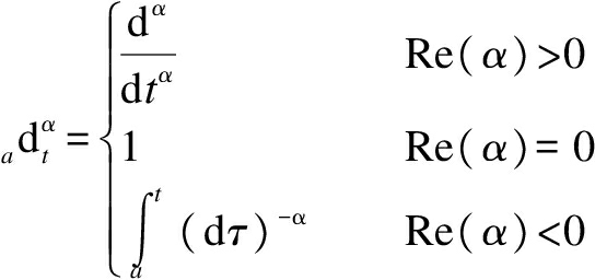
(1)
where Re(α)is the real part of α.
So far, fractional calculus has no uniform definition.In the development of fractional calculus, there are several definitions of fractional calculus.Three most commonly used definitions are Caputo, Riemann-Liouville (RL)and Grumwald-Letnikov (GL)[19].For example, the definition of GL is defined as

(2)

(3)
where Γ(·)is the Gamma function; [(t-a)/h] is the largest integer that is not greater than (t-a)/h, and h is the sampling period.
1.2 Fractional-order systems
Conventionally, integer-order calculus is used to describe natural phenomena, but many phenomena in nature cannot be accurately described by the traditional integer-order differential equations.Therefore, it is necessary to extend the traditional calculus to describe such phenomena.Fractional differential equation is an extension of traditional calculus, which can describe complex physical systems more accurately.
The general expression of the SISO linear fractional-order system differential equation is shown below.
anDαny(t)+an-1Dαn-1y(t)+…+a0y(t)=
bmDβmu(t)+bm-1Dβm-1u(t)+…+b0u(t)
(4)
where ai and bi are real numbers; αi and βi are calculus orders; u(t)and y(t)are the input and output signals of the system, respectively.Under a zero initial condition, the expression of the transfer function is described as
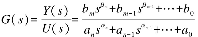
(5)
At present, it is difficult to identify the general fractional-order system, because it is difficult to determine the order of the system.In Ref.[20], the concept of continuous order distribution was proposed, and the general expression of the fractional-order system was transformed into an expression with common factor order, which is shown below.
anDnαy(t)+an-1D(n-1)αy(t)+…+a0y(t)=
bmDmβu(t)+bm-1D(m-1)βu(t)+…+b0u(t)
(6)
The corresponding transfer function is
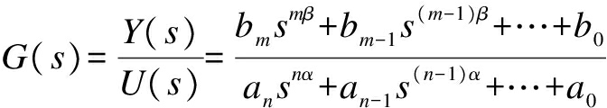
(7)
1.3 PSO variants
1.3.1 ACPSO algorithm
PSO is a new evolutionary algorithm, which seeks for the optimal solution by sharing information among individuals.In the process of optimization, each particle updates its velocity and position as follows[15]:
vi(t+1)=wvi(t)+c1r1(Pi(t)-xi(t))+c2r2(G(t)-xi(t))
(8)
xi(t+1)=xi(t)+vi(t+1)
(9)
where w is the inertia weight; vi(t)is the velocity of particle i at iteration t; c1 and c2 are two positive constants between 0 and 1; r1 and r2 are two random numbers between 0 and 1; Pi(t)is the optimum value of particle i at iteration t;xi(t)is the current position of particle i at iteration t; G(t)is the optimum value of the particle population.
In Ref.[14], a linearly decreasing inertia weight strategy was introduced in conventional PSO.The modified inertia weight w is shown below.

(10)
The corresponding velocity updating formula is
vi(t+1)=w(t)vi(t)+c1r1(Pi(t)-xi(t))+
c2r2(G(t)-xi(t))
(11)
where wmax is the maximum value of inertia weight w; wmin is the minimum value of inertia weight w; T is the maximum number of iterations.Usually, the inertia weight w is set from 0.9 to 0.4[21].
In Ref.[17], in order to improve the convergence rate of PSO, the ACPSO is proposed, which is expressed as
vi(t+1)=![]() +
+
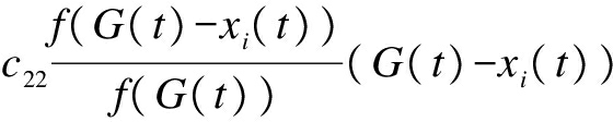
(12)
where f(Pi(t))is the best fitness function found by the i-th particle at iteration t;f(G(t))is the best objective function found by the swarm up to the iteration t.With this method, the velocity can be updated adaptively, which accelerates the convergence of the algorithm.
1.3.2 IPSO algorithm
The classical PSO algorithm only uses the individual optimal value and the optimal value of the population, and does not take into account the information of other individuals in the population.With this in mind, an improved PSO with the passive congregation was proposed in Ref.[18].The velocity updating of the IPSO algorithm is shown as
vi(t+1)=w(t)vi(t)+c1r1(Pi(t)-xi(t))+
c2r2(G(t)-xi(t))+c3r3(P(t)-xi(t))
(13)
where P(t)is the current position of a random particle at iteration t.The introduction of the passive congregation can further increase the information exchange between groups, so that the population can find the optimal value more quickly.
2 Proposed MPSO Algorithm
In order to increase the exchange of information among individuals, and make full use of the information in the population, so as to improve the search speed and avoid the local optimum, the average value of position is introduced in this paper.Furthermore, in order to avoid the extreme value existing in the position information, a modified Tent mapping is proposed.
2.1 Modified Tent mapping
Tent mapping is a type of piecewise linear one-dimensional chaotic mapping, which has the advantages of simple form, uniform power spectrum density and good correlation properties.Compared with other chaotic sequences, such as logistics sequence, the improved Tent mapping has better uniformity and is more suitable for computer digital computation.The recursive formula of Tent mapping is
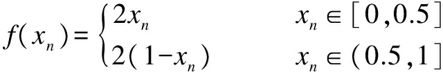
(14)
There are small cycles and some unstable periodic points in the Tent sequence, e.g.(0.2, 0.4, 0.8, 0.6)and (0.25, 0.5, 0.75).In order to prevent the iterations from falling into the small cycles, we design the modified sequence generation method.The specific steps are as follows.
1)Take a point x0 that does not fall into the small cycle, and set z(1)=x0, i=j=1.
2)Generate sequence x according to Eq.(14), i=i+1.
3)Suppose that the maximum iteration number is M1, if i>M1, then execute Step 5); else if x(i)∈{0,0.25,0.5,0.75} or x(i)=x(i-k), k∈{0,1,2,3,4}, then return to Step 4), else return to Step 2).
4)Change the initial value of iteration: x(i)=z(j+1)=z(j)+ε, j=j+1, return to Step 2).
5)Terminate the operation and save sequence x.
The initial value and the iteration number are set to be 0.435 8 and 1 000, respectively.Fig.1 shows the generated sequence x.

Fig.1 The generated sequence diagram
2.2 MPSO algorithm
Suppose that the number of particles is N, the specific steps of the Tent chaotic search are shown below.
1)The average value M of position is obtained, and the definition of M is
2)The optimization variables from the interval [a, b] are transformed into chaotic variables z from the interval [0, 1],
zi=(Mi-a)/(b-a) i=1,2,…,D
where D is the number of variable dimensions.
3)N iterations are executed to generate ![]() according to the generation method of chaotic sequence in Section 2.1, n=1,2,…,N.
according to the generation method of chaotic sequence in Section 2.1, n=1,2,…,N.
4)The chaotic sequence is translated to the original variable range as follows:

Then, N feasible solutions can be obtained by
5)The average value is calculated as

The velocity updating of the MPSO algorithm is shown as
vi(t+1)=w(t)vi(t)+c1r1(Pi(t)-xi(t))+
c2r2(G(t)-xi(t))+c3r3(Pav(t)-xi(t))
(15)
The inertia weight w in Eq.(15)is updated according to Eq.(10), and the position is updated according to Eq.(9).
2.3 Performance evaluation
2.3.1 Classical test functions
In the test stage, eight classical test functions are introduced to test the performance of the MPSO and other algorithms as follows:
Ackley

Schewefel

Rastrigrin function
Griewank function

Rosenbrock function

Sphere function
Sum squares

Dixon-price

f1 to f8 have a common global minimum.Besides, f1 to f4 are multimodal test functions, while f5 to f8 are unimodal test functions.Unlike the unimodal test functions, the number of local optimal values in the multimodal test functions increases with the increase of the dimension.The basic information of the eight test functions is listed in Tab.1.
Tab.1 Basic information of the test functions

FunctionDimensionSolutionspaceOptimalvaluef130[-100,100]D0f230[-500,500]D0f330[-100,100]D0f430[-100,100]D0f530[-10,10]D0f630[-10,10]D0f730[-10,10]D0f830[-10,10]D0
2.3.2 Parameter analysis
In the MPSO algorithm, the selection of c3 influences the performance of the algorithm.In order to analyze the effect of c3 on the performance of the algorithm, four multimodal functions f1 to f4 and two unimodal functions f5 and f6 are used to test the algorithm with different c3 values.In the MPSO algorithm, the population size N is set to be 50; the inertia weight w adopts the linear decreasing strategy in Ref.[14], and its variation range is 0.7-0.9; the learning factors c1 and c2 are set to be 0.5-10.The test results for c3 are shown in Tab.2.
Tab.2 Average fitness values of functions f1-f6 with different c3
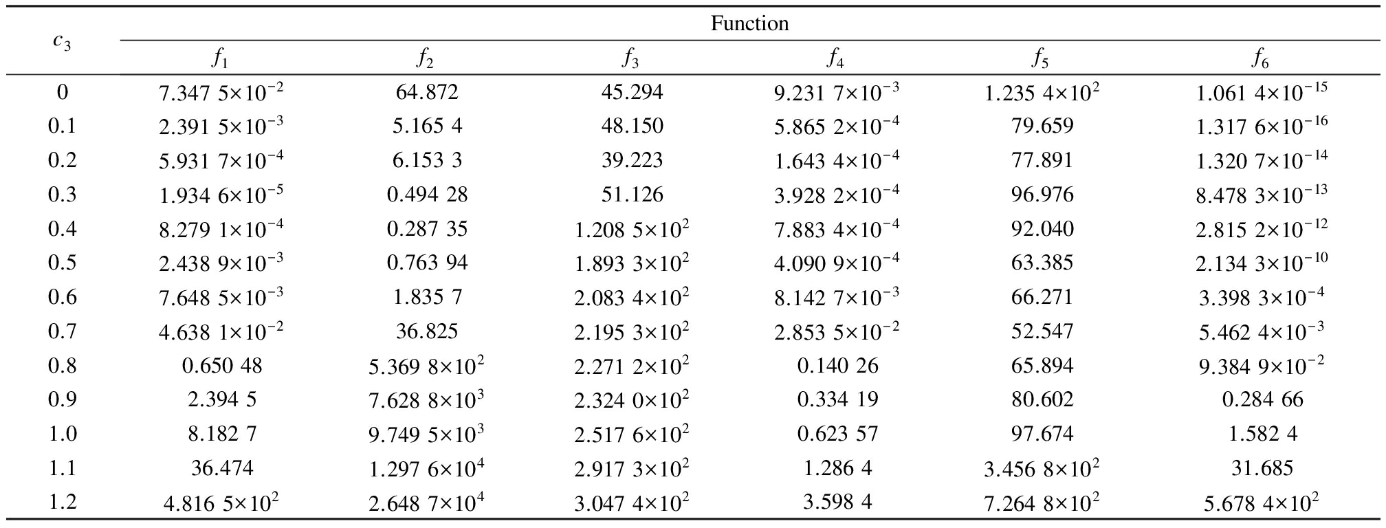
c3Functionf1f2f3f4f5f607.3475×10-264.87245.2949.2317×10-31.2354×1021.0614×10-150.12.3915×10-35.165448.1505.8652×10-479.6591.3176×10-160.25.9317×10-46.153339.2231.6434×10-477.8911.3207×10-140.31.9346×10-50.4942851.1263.9282×10-496.9768.4783×10-130.48.2791×10-40.287351.2085×1027.8834×10-492.0402.8152×10-120.52.4389×10-30.763941.8933×1024.0909×10-463.3852.1343×10-100.67.6485×10-31.83572.0834×1028.1427×10-366.2713.3983×10-40.74.6381×10-236.8252.1953×1022.8535×10-252.5475.4624×10-30.80.650485.3698×1022.2712×1020.1402665.8949.3849×10-20.92.39457.6288×1032.3240×1020.3341980.6020.284661.08.18279.7495×1032.5176×1020.6235797.6741.58241.136.4741.2976×1042.9173×1021.28643.4568×10231.6851.24.8165×1022.6487×1043.0474×1023.59847.2648×1025.6784×102
From Tab.2, it can be seen that MPSO obtains good results on function f1 when c3=0.3.The best result for function f2 is obtained when c3=0.4.MPSO obtains good results on function f6 when c3=0.1.For function f5, the best result is obtained when c3=0.7.With c3=0.2, MPSO obtains the best results for functions f3 and f4.The test results of MPSO on function f4 and f6 deteriorate with c3≥0.8.Considering the situation mentioned above, the value range of c3 is set to be 0.1-0.7.
2.3.3 Evaluation results
The population size of all the algorithms is set to be 50.For the GA algorithm, the crossover and mutation probabilities are Pc=0.7 and Pm=0.15, respectively.For the IPSO algorithm, the learning factors c1 and c2 are set to be 0.5, and the inertia weight w is set to be [0.7, 0.9].For the ACPSO algorithm, the learning factors c1 and c2 are set to be 2, and the inertia weight w is the same as that in Ref.[18].The proposed MPSO algorithm is tested by the classical test functions f1 to f8, and is compared with GA, IPSO and ACPSO algorithms.The maximum number of iterations is 1 000.In order to make the results more convincing, 100 experiments were carried out.The mean, the standard deviations(SD)and the average number of iterations (Iter)of the test results are listed in Tab.3.
Tab.3 Performance comparisons of MPSO, ACPSO, IPSO and GA algorithms

FunctionGAMean(SD)IterIPSOMean(SD)IterACPSOMean(SD)IterMPSOMean(SD)Iterf10.58347(0.92864)2560.25378(0.48367)2017.7281×10-3(1.3592×10-2)1752.2475×10-5(5.6137×10-5)186f24.2841×103(7.4825×103)1831.7629×103(2.9674×103)961.1862×102(2.8573×102)800.37286(0.78648)83f31.6053×102(1.8820×102)2861.0512×102(1.4522×102)13528.955(30.848)1177.5067×10-2(0.17909)128f40.37498(0.27988)2470.19124(0.21611)1621.3836×10-2(1.8368×10⁻²)1451.6576×10-5(2.1719×10⁻⁵)149f51.4467×103(6.1225×10³)2192.6721×102(8.4294×10²)12823.034(52.787)1021.48452(2.42025)108f64.3288×10-3(9.5167×10-3)1861.5978×10-5(6.3265×10-5)1342.2406×10-8(7.5161×10-8)822.3412×10-10(4.4798×10-10)97f73.5213(7.4734)2820.23175(0.78244)2014.0738×10-2(8.3417×10-2)1572.6424×10-3(6.3275×10-3)164f82.5197×102(7.6274×102)30257.162(1.1384×102)1730.65372(0.98672)1310.10517(0.31216)137
From Tab.3, compared with GA and IPSO algorithms, it can be clearly found that the MPSO algorithm has better performance in terms of both the mean and standard deviation.Compared with the ACPSO algorithm, the overall convergence rate of MPSO is relatively slow, but the MPSO algorithm has better convergence precision.One reason is that the ACPSO algorithm uses an adaptive learning factor, which can speed up the convergence rate of the algorithm.On the other hand, the proposed MPSO algorithm increases the information exchange among individuals in the population, and can search the solution space more carefully, so as to achieve better convergence precision.
In conclusion, the introduction of the average value of position takes full advantage of the information in the population, and the application of Tent mapping avoids the emergence of extreme values, which improves the convergence precision and the searching efficiency of the MPSO algorithm.
3 Simulations
To demonstrate the effectiveness of the proposed MPSO algorithm, based on the systems with known model structures and unknown model structures, the MPSO algorithm is compared with some typical algorithms, including GA, IPSO and ACPSO algorithms.The basic parameter settings are similar to the settings in Section 2.3.Only considering the influence of population size (PN)on time complexity, the analysis of time complexity for the proposed MPSO algorithm and other algorithms being compared in a single run is concluded as follows: For the MPSO algorithm, the time complexity for the initialization process is O(PN); the time complexity for calculating the objective function values is O(PN); the time complexity for updating and selecting the individual and global optimal values is O(PN); the time complexity for calculating the mean of the position information in passive congregation terms is O(PN); the time complexity for updating the location information of particles using Tent mapping is O(PN); the time complexity for generating new velocities and positions is O(PN).Thus, the overall time complexity of the MPSO algorithm in one iteration is: O(PN)+O(PN)+O(PN)+O(PN)+O(PN)+O(PN), which can be regarded as O(MPSO)=O(PN).For the GA algorithm, the time complexity is mainly composed of roulette wheel selection, crossover and mutation operations, and the corresponding time complexities are ![]() O(PN)and O(PN), respectively.Therefore, the time complexity of the GA algorithm can be simplified as
O(PN)and O(PN), respectively.Therefore, the time complexity of the GA algorithm can be simplified as ![]() Similarly, the time complexities of the IPSO and ACPSO algorithms are O(PN)and O(PN), respectively.In short, we can conclude that O(GA)>O(MPSO)
Similarly, the time complexities of the IPSO and ACPSO algorithms are O(PN)and O(PN), respectively.In short, we can conclude that O(GA)>O(MPSO) O(IPSO)O(ACPSO).
The simulations are implemented using MATLAB 7.11 on Intel(R)Core(TM)i5-2320 CPU, 3.00 GHz with 4 GB RAM.The specific identification steps are as follows.
1)Determine the vector to be searched (model parameters and order).
2)Determine the performance index (evaluation function).In this paper, the step signal is introduced to be as the input signal.The sum of the squared errors between the output y(t)and the true value y0(t), i.e.,
J=![]() is used as the performance evaluation function.
is used as the performance evaluation function.
3)The parameters of the algorithm are initialized to generate random search vectors.
4)According to the steps of the MPSO algorithm, the parameters in the fractional-order system are identified.
5)The iteration is repeated until the performance index is satisfactory.Output the identification results.
The schematic diagram of parameter estimation for the fractional-order system is shown in Fig.2.

Fig.2 Schematic diagram of parameter estimation for the fractional-order system
3.1 Identification of known fractional-order model structure
Assume that the transfer function of the identified object is

(16)
The range of parameters is set to be [0, 3], and the random number for the model order changes from -0.05 to 0.05.The identification vector is defined as
x=[a1 a2 a3 b1 b2]
where a1,a2,a3 are the model parameters and b1,b2 are the orders of the model.The statistical results of the best, the mean and the worst estimated parameters over 20 independent runs are shown in Tab.4.
We can see from Tab.4 that the obtained estimated values by MPSO are closer to the true values, which shows that the MPSO algorithm is more accurate than GA, IPSO and ACPSO algorithms.Furthermore, it can also be easily found that the best objective function values obtained by MPSO are better than those obtained by other algorithms.
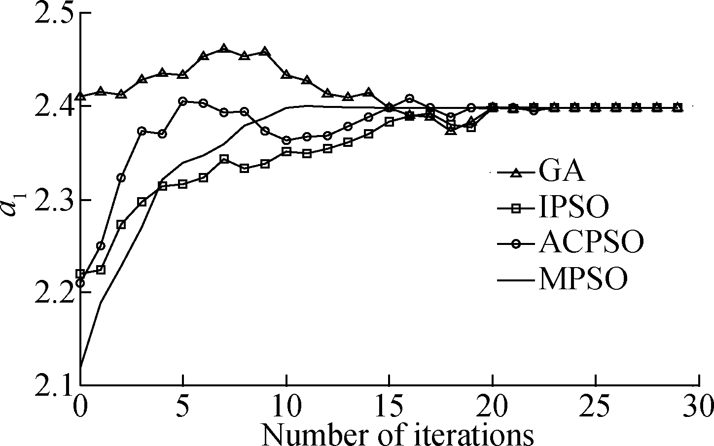
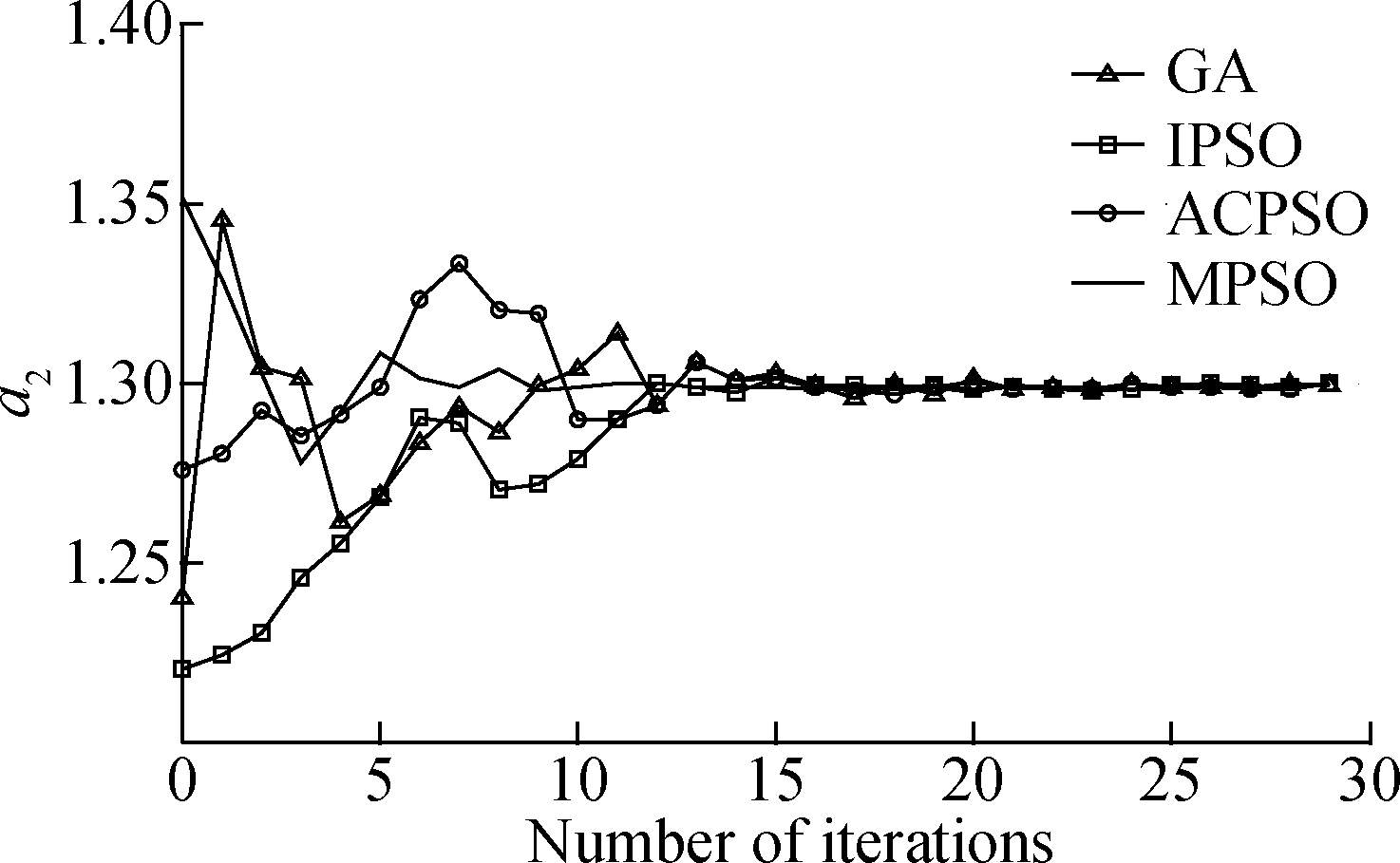
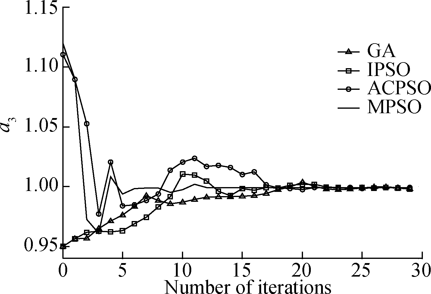
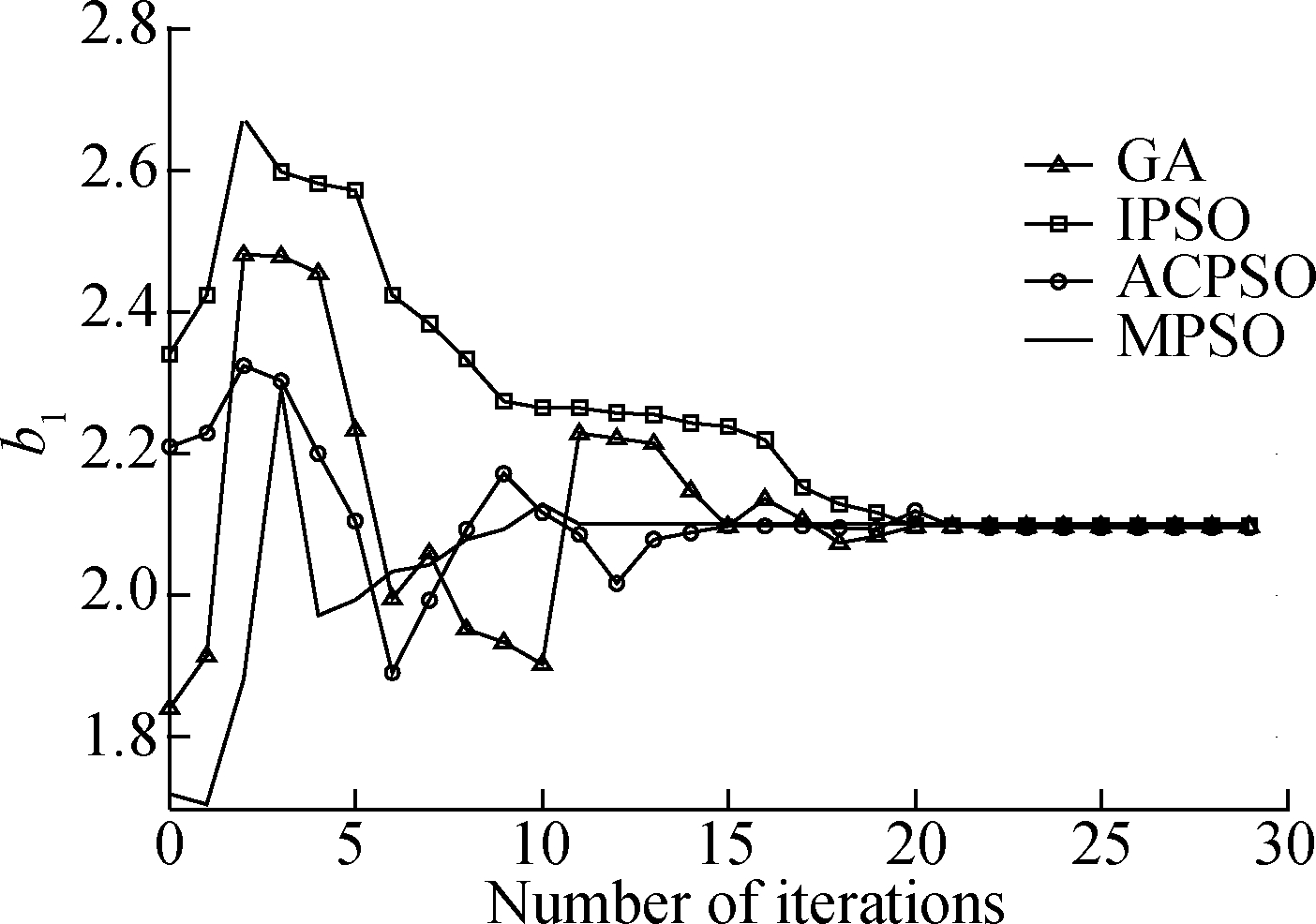
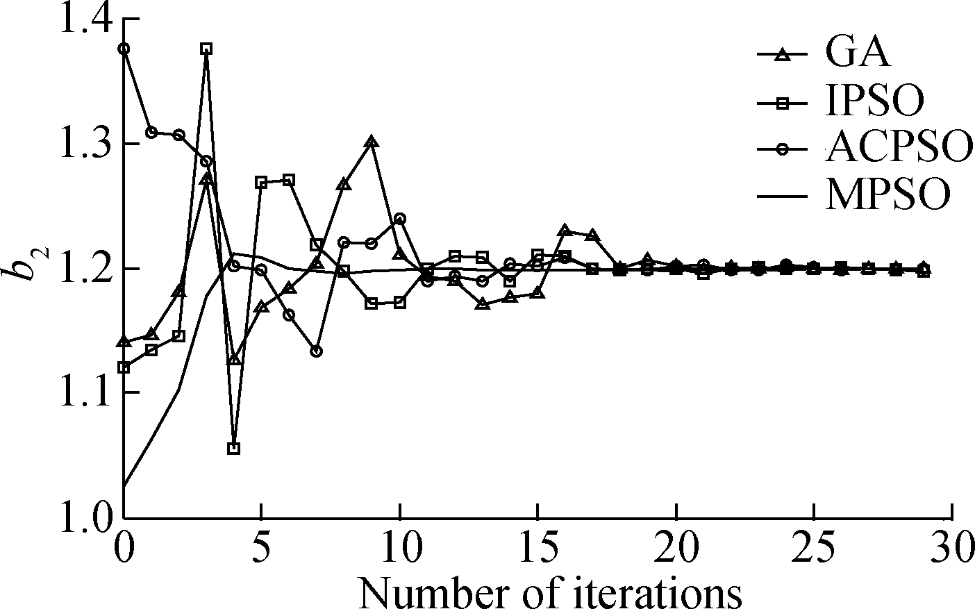
The estimated parameters generated by various algorithms in a single run are shown in Fig.3.Fig.3 reveals that the performance of the MPSO algorithm surpasses the IPSO algorithm due to the full use of information among individuals.Moreover, in the early stage of evolution, the convergence rate of the ACPSO algorithm is slightly faster due to the introduction of an adaptive learning factor.However, the estimated parameters generated by MPSO yield a better precision as compared to that of other comparison algorithms, which suggests that our presented algorithm is more susceptible to a small change in parameters.
(a)
(b)
(c)
(d)
(e)
Fig.3 Evolutionary curve of parameters estimation.(a)a1;(b)a2; (c)a3; (d)b1; (e)b2
Tab.4 The estimation results of various algorithms for Eq.(16)

AlgorithmGAIPSOACPSOMPSOa12.38102.38482.38972.3982a21.29541.29701.29821.2998Besta30.99020.99110.99430.9994b12.08892.08992.09502.0999b21.19451.19501.19821.1996J0.24510.20947.8204×10-26.4068×10⁻⁴a12.37522.37912.38532.3948a21.27101.27981.28621.2987Meana30.98260.98470.99580.9982b12.07432.07812.09012.0981b21.18071.18581.19481.1982J0.73320.59334.8415×10-27.7014×10⁻³a12.35272.35992.38292.4117a21.26371.27511.28351.2838Worsta30.97750.98170.99420.9964b12.06562.07362.08722.0964b21.17841.18031.19261.1914J1.24720.83619.3503×10-21.7815×10-2
Moreover, considering the time complexity, we can easily see that the MPSO algorithm outperforms the GA algorithm whether in the convergence characteristics or in the time complexity.In addition, under the same level of time complexity with the IPSO and ACPSO algorithms, the MPSO algorithm has a better convergence rate and accuracy.
In order to study the influence of the variation range of order on the identification, the variation range of order is set to be [-0.5, 0.5], and other conditions remain unchanged.The statistical results are shown in Tab.5.
From Tab.5, we can see that the identification effect can be improved significantly with the decrease of the random number range of order.The main reason is that the objective function value affected by the order changes exponentially, which indicates that there is a significant change in the function value with a minor change of order.Therefore, the appropriate reduction of the order helps to shorten the convergence time of the algorithm and improve search ability.
3.2 Identification for unknown fractional-order model structure
In the model identification, the model structure is often unknown.When the assumed model structure matches the real model, the error is smaller than that of other models.In the actual identification, the high-order system is relatively small, and the higher order fractional-order system can be reduced to one of the models in Tab.6.Therefore, the three models in Tab.6 are selected for simulation study.Assume that the transfer function of the identified object is
Tab.5 The estimation results of various algorithms for Eq.(16)

AlgorithmGAIPSOACPSOMPSOa12.27182.28372.29082.3547a21.11671.12871.13841.1821Besta30.93370.94370.94840.9923b11.92681.94711.97752.0357b21.06321.07681.09371.1685J14.138010.60307.65710.4920a12.20952.21462.21782.3219a21.05131.05181.12761.1672Meana30.89270.90370.94090.9892b11.95161.95201.96072.0263b21.04971.05281.08941.1446J24.489021.098011.14801.3132a11.98082.02732.11382.2121a20.98680.99541.08741.1485Worsta30.87370.89760.92750.9547b11.85821.87231.91061.9371b20.97570.98281.09721.1154J37.857026.896015.80409.2557
(17)
Tab.6 The model structure

ModelStructureParameter11a1Sb1+a2a1,a2,b121a1Sb1+a2Sb2+a3a1,a2,a3,b1,b231a1Sb1+a2Sb2+a3Sb3+a4a1,a2,a3,a4,b1,b2,b341a1Sb1+a2Sb2+a3Sb3+a4Sb4+a5a1,a2,a3,a4,a5,b1,b2,b3,b4
The statistical results are shown in Tab.7.From Tab.7, we notice that the MPSO algorithm outperforms other algorithms being compared.In addition, we can also find that the performance index J of model 3 is significantly small, so model 3 is the closest to the target.In addition, taking the J value of model 3 as the dividing point, the J value decreases first and then increases.Furthermore, it is clear that the difficulty of parameter identification greatly increases with the increase in the number of the parameters in the system.
4 Conclusions
1)A new parameter identification scheme based on a modified PSO algorithm is proposed.The introduction of the average value of position information makes full use of the information exchange among individuals in the population, which can improve the precision and efficiency of optimization.By utilizing the uniformity and ergodicity of Tent mapping, MPSO can avoid the extreme value of position information, so as not to fall into local optimal values.
Tab.7 The estimation results of various algorithms for Eq.(17)
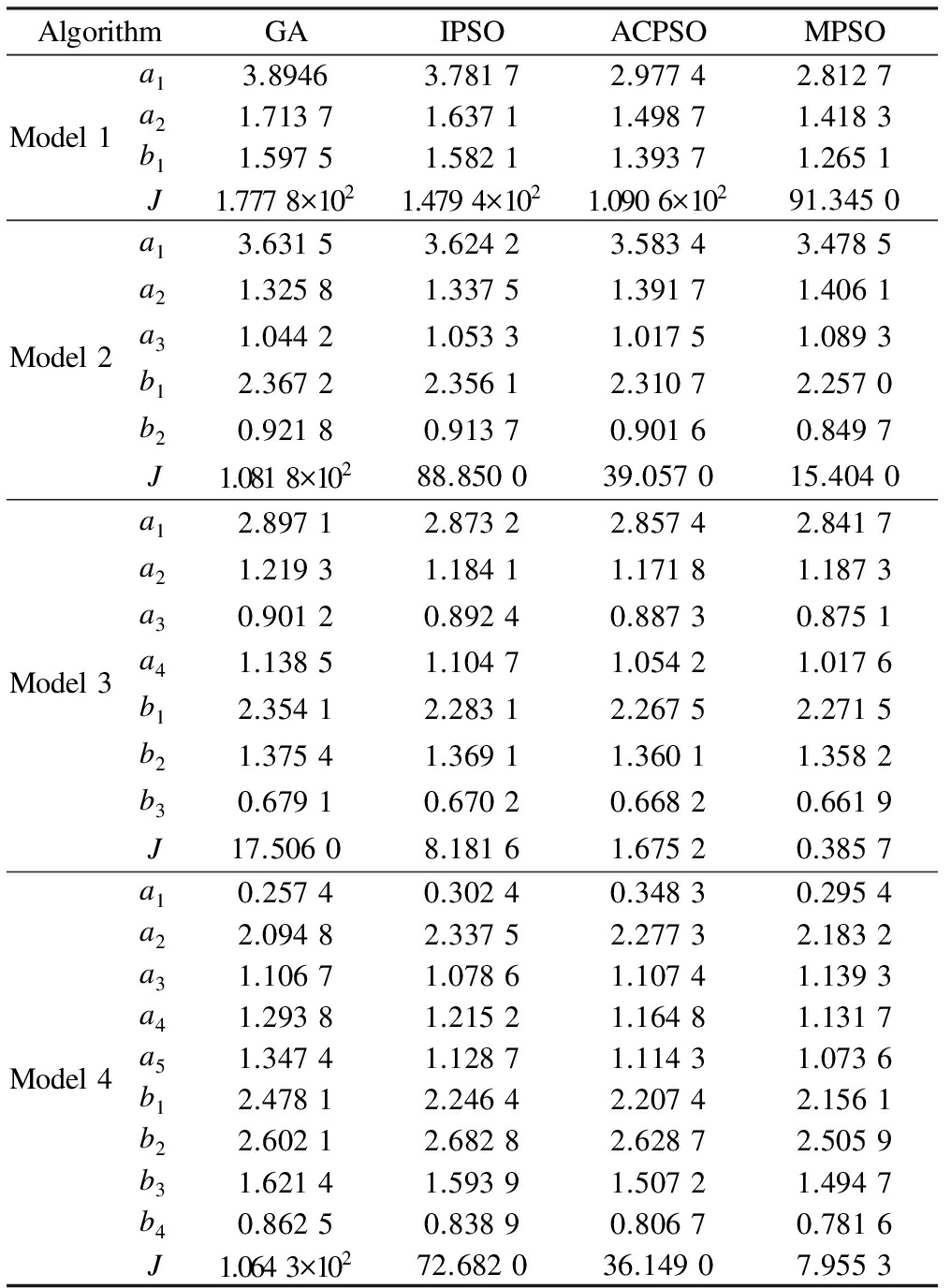
AlgorithmGAIPSOACPSOMPSOa13.89463.78172.97742.8127Model1a21.71371.63711.49871.4183b11.59751.58211.39371.2651J1.7778×1021.4794×1021.0906×10291.3450a13.63153.62423.58343.4785a21.32581.33751.39171.4061Model2a31.04421.05331.01751.0893b12.36722.35612.31072.2570b20.92180.91370.90160.8497J1.0818×10288.850039.057015.4040a12.89712.87322.85742.8417a21.21931.18411.17181.1873a30.90120.89240.88730.8751Model3a41.13851.10471.05421.0176b12.35412.28312.26752.2715b21.37541.36911.36011.3582b30.67910.67020.66820.6619J17.50608.18161.67520.3857a10.25740.30240.34830.2954a22.09482.33752.27732.1832a31.10671.07861.10741.1393a41.29381.21521.16481.1317Model4a51.34741.12871.11431.0736b12.47812.24642.20742.1561b22.60212.68282.62872.5059b31.62141.59391.50721.4947b40.86250.83890.80670.7816J1.0643×10272.682036.14907.9553
2)Compared with the other three algorithms, the identification results verify the fine searching capability and efficiency of the presented algorithm.For the systems with known model structures and unknown model structures, the proposed approach can obtain the estimated parameters with a faster convergence rate and higher convergence precision.
3)In conclusion, the proposed MPSO algorithm is an efficient and promising approach for parameter identification of the fractional-order system.
We mainly study the fractional-order linear model with constant coefficient in this paper.In future work, we will further study the parameter identification of the fractional-order system which contains nonlinearity models and input signals with fractional differential components.
References
[1]Diethelm K.An efficient parallel algorithm for the numerical solution of fractional differential equations[J].Fractional Calculus and Applied Analysis, 2011, 14(3): 475-490.DOI:10.2478/s13540-011-0029-1.
[2]Gepreel K A.Explicit Jacobi elliptic exact solutions for nonlinear partial fractional differential equations [J].Advances in Difference Equations, 2014, 2014(1): 1-14.DOI:10.1186/1687-1847-2014-286.
[3]Laskin N.Fractional market dynamics[J].Physica A: Statistical Mechanics and Its Applications, 2000, 287(3): 482-492.DOI:10.1016/s0378-4371(00)00387-3.
[4]Ionescu C, Machado J T, de Keyser R.Fractional-order impulse response of the respiratory system[J].Computers & Mathematics with Applications, 2011, 62(3): 845-854.DOI:10.1016/j.camwa.2011.04.021.
[5]Badri V, Tavazoei M S.Fractional order control of thermal systems: Achievability of frequency-domain requirements[J].Nonlinear Dynamics, 2014, 80(4): 1773-1783.DOI:10.1007/s11071-014-1394-1.
[6]Vikhram Y R, Srinivasan L.Decentralised wide-area fractional order damping controller for a large-scale power system[J].IET Generation, Transmission & Distribution, 2016, 10(5): 1164-1178.DOI:10.1049/iet-gtd.2015.0747.
[7]Safarinejadian B, Asad M, Sadeghi M S.Simultaneous state estimation and parameter identification in linear fractional order systems using coloured measurement noise [J].International Journal of Control, 2016, 89(11): 2277-2296.
[8]Taleb M A, Béthoux O, Godoy E.Identification of a PEMFC fractional order model[J].International Journal of Hydrogen Energy, 2017, 42(2): 1499-1509.DOI:10.1016/j.ijhydene.2016.07.056.
[9]Storn R, Price K.Differential evolution—A simple and efficient heuristic for global optimization over continuous spaces [J].Journal of Global Optimization, 1997, 11(4): 341-359.
[10]Tao C, Zhang Y, Jiang J J.Estimating system parameters from chaotic time series with synchronization optimized by a genetic algorithm [J].Physical Review E, 2007, 76(2): 016209.DOI:10.1103/PhysRevE.76.016209.
[11]Kennedy J, Eberhart R.Particle swarm optimization[J].Proceedings of ICNN’95—International Conference on Neural Networks.Perth, Australia, 1995: 1942-1948.DOI:10.1109/icnn.1995.488968.
[12]Gupta R, Gairola S, Diwiedi S.Fractional order system identification and controller design using PSO [C]//2014 Innovative Applications of Computational Intelligence on Power, Energy and Controls with Their Impact on Humanity.Ghaziabad, India, 2015: 149-153.DOI:10.1109/cipech.2014.7019053.
[13]Hammar K, Djamah T, Bettayeb M.Fractional hammerstein system identification using particle swarm optimization [C]//2015 7th IEEE International Conference on Modelling, Identification and Control.Sousse, Tunisia, 2015: 1-6.DOI:10.1109/icmic.2015.7409483.
[14]Shi Y, Eberhart R C.A modified particle swarm optimizer [C]//1998 IEEE International Conference on Evolutionary Computation.Anchorage, USA, 1998: 69-73.DOI:10.1109/icec.1998.699146.
[15]Koulinas G, Kotsikas L, Anagnostopoulos K.A particle swarm optimization based hyper-heuristic algorithm for the classic resource constrained project scheduling problem [J].Information Sciences, 2014, 277: 680-693.DOI:10.1016/j.ins.2014.02.155.
[16]Gong Y J, Li J J, Zhou Y, et al.Genetic learning particle swarm optimization[J].IEEE Trans Cybern, 2016, 46(10): 2277-2290.DOI:10.1109/TCYB.2015.2475174.
[17]Aghababa M P.Optimal design of fractional-order PID controller for five bar linkage robot using a new particle swarm optimization algorithm[J].Soft Computing, 2016, 20(10): 4055-4067.DOI:10.1007/s00500-015-1741-2.
[18]He S, Wu Q H, Wen J Y, et al.A particle swarm optimizer with passive congregation[J].Biosystems, 2004, 78(1/2/3): 135-147.DOI:10.1016/j.biosystems.2004.08.003.
[19]Rossikhin Y A, Shitikova M V.Application of fractional calculus for dynamic problems of solid mechanics: Novel trends and recent results [J].Applied Mechanics Reviews, 2009, 63(1): 010801.DOI:10.1115/1.4000563.
[20]Hartley T T, Lorenzo C F.Fractional-order system identification based on continuous order-distributions[J].Signal Processing, 2003, 83(11): 2287-2300.DOI:10.1016/s0165-1684(03)00182-8.
[21]Gaing Z L.A particle swarm optimization approach for optimum design of PID controller in AVR system[J].IEEE Transactions on Energy Conversion, 2004, 19(2): 384-391.DOI:10.1109/tec.2003.821821.