Recently, the neural network (NN) models have attracted attention from researchers working on power amplifier (PA) modeling due to their successful implementation in pattern recognition, signal processing, system identification, and control[1-2]. Different neural topologies have been proposed. For example, the complex-valued single-input single-output feed-forward NN[3] and real-valued double-input double-output NN[4] are the most basic structures. These NNs have been found effective for forward modeling of static nonlinear PAs. However, these models do not consider the memory effects of PAs, especially when the PAs have a strong memory effect, these models fall short of expectation.
Considering the memory effect, three dynamic neural structures have been proposed in the NN literature, namely, the recurrent neural network[5], the complex-valued time-delay neural network (TDNN)[6] and the real-valued focused time-delay neural network[7]. The recurrent neural network employs the feed-forward and the feedback complex-valued time-delay line, but the feedback time-delay line significantly affects model robustness. Present and past complex signals are used to train the time-delay neural network, but they cannot be used to describe the strongly nonlinearity of Doherty PA. The memory effect is considered in real-valued TDNN, and the present and past inputs of the real-valued TDNN are real-valued. However, the real-valued TDNN has several hidden layers, and it is a back-propagation NN that demands a lengthy training time.
In this paper, a real and complex-valued hybrid TDNN is proposed, simply called hybrid TDNN. In this hybrid NN, the generalized memory effect[8] of input signals is considered. The inputs to the hybrid TDNN are complex-valued signals and the fractional order of the complex-valued signal module. The hybrid TDNN is based on the radial basis function (RBF), so it has only one hidden layer, which greatly reduces computational complexity and training time. Moreover, it has better modeling and linearization capability.
1 Nonlinear Model of Hybrid TDNN
PA modeling calls for a model that can extract magnitude and phase information from modulated complex waveforms. To address cumbersome calculations and describe static nonlinear PAs, the real-valued feed-forward neural network[9] is shown in Fig.1, which takes advantage of the in-phase (I) and quadrature (Q) components of modulated waveforms in the baseband, thereby saving pre- and post-processing activities, and it can be used as a common feed-forward NN with two inputs and two outputs. Although this topology has been found to be effective for forward modeling of static nonlinear PAs, it falls short of expectation when the PA shows memory effect. Usually, the memory effect of the PA cannot be ignored[10-11], especially in the case of wideband signals.

Fig.1 Real-valued NN topologies for RF PA modeling
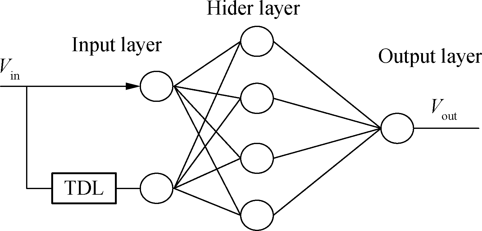
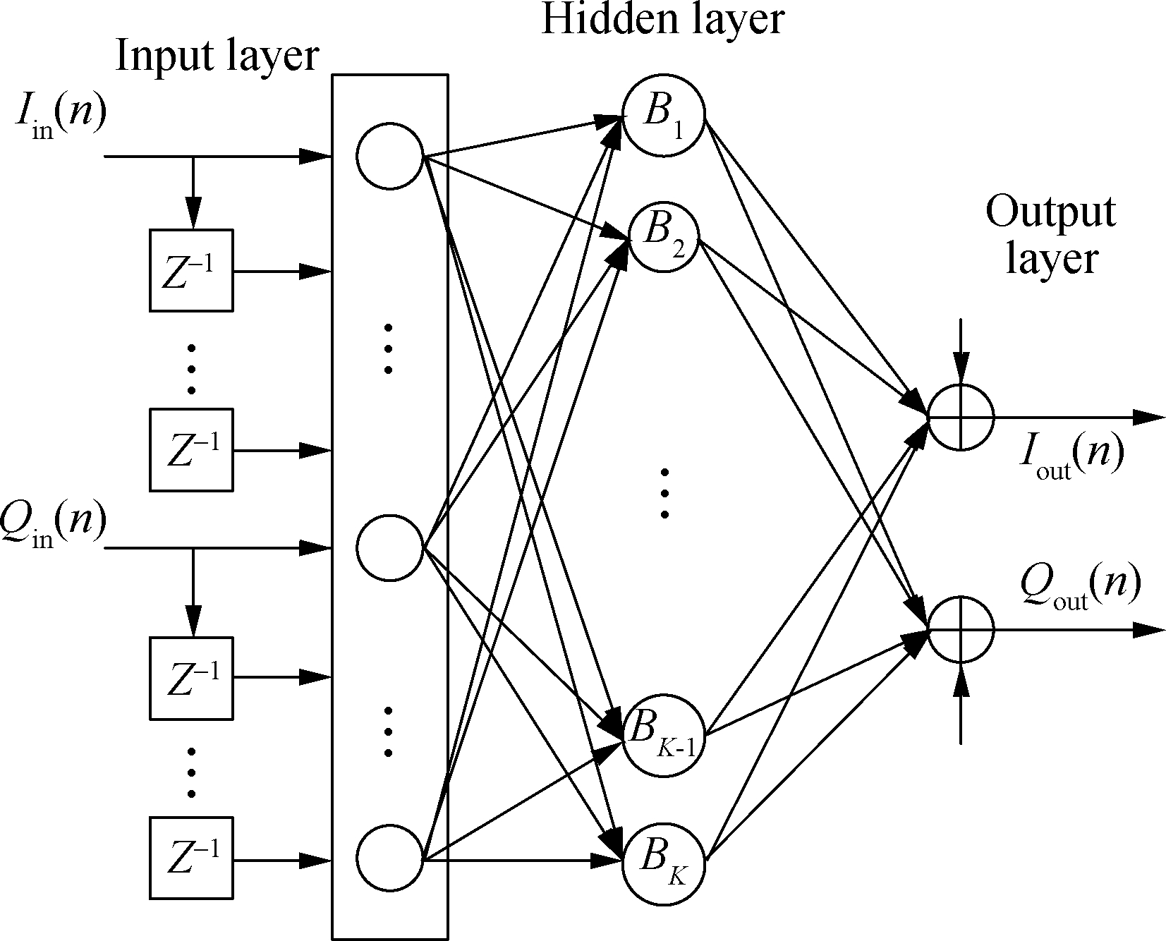
Considering the memory effect, two dynamic neural structures have been proposed in NN literature. First, the complex-valued TDNN[6] that utilizes feed-forward signal processing is shown in Fig.2(a). It uses complex baseband signals as the model input and output. The second technique is a real-valued focused TDNN[7] that relies on the fact that the amplifier output depends on present, as well as previous input values owing to memory effect in the system. Thus, this technique extracts information from present and past inputs. To reduce the number of hidden layers of the real-valued TDNN, an real-valued TDNN-based RBF is used[12], namely, real-valued time-delay RBF NN, and its topology is shown in Fig.2(b). However, this scheme does not consider the generalized memory effect and the module of the baseband signal. Therefore, it cannot accurately describe the strong nonlinearities of power amplifiers.
(a)
(b)
Fig.2 Two different topology of NN models. (a) Topology of complex-valued TDNN model. (b) Topology of real-valued time delay RBF NN
To address this issue,a new topology of the RBF NN, the real and complex-hybrid TDNN is proposed in this paper. It contains complex and real-valued inputs, where the complex-valued inputs are complex baseband data and the real-valued inputs are fractional orders of the complex-valued signal module. Moreover, the generalized memory effect is considered in the model; that is, the output of the complex baseband data depends on leading time, aligned time and past time values.
1.1 Topology of hybrid TDNN nonlinear model
According to Ref.[8], the generalized memory polynomial (GMP) model and the traditional memory polynomial (MP) model are given. These models originate from the Volterra series, and the outputs of these models depend on the complex baseband signal and module value of the complex value signal. They are given as
y(n)=![]()
(1)
(2)
where y(n) depends on the present and past time complex baseband signals x(n-l),l∈[0,1,2,…]; the order of the present and the past time complex baseband signal module values is |x(n-l)|k,l∈[0,1,2,…]; and the order of leading time complex baseband signal module values is |x(n+l)|k,l∈[1,2,…].
The NN model is known as a black box, which can be described by the function f(x), the input and output of which are selected to describe the nonlinearity of the PA. Based on the above mentioned characteristics of the GMP and the MP model, the input data of an NN model includes present and past time complex baseband signals, the order of the present and the past time complex baseband signal module values, and the order of leading time complex baseband signal module values.
For the RBF NN model, the basis function is a Gaussian function[12], and the input data of the model is used in the Gaussian function. Therefore, if x(n-l), |x(n-l)|k, and |x(n+l)|k are used as the inputs to the RBF NN model, x(n-l), x(n-l)2, |x(n-l)|k, |x(n-l)|2k, and |x(n+l)|k and |x(n+l)|2k are used in the Gaussian function. In Ref.[13], the odd-order nonlinearity is the main nonlinearity of the PA. In Ref.[8], the fractional order and odd-order nonlinearity are simultaneously considered to increase modeling accuracy. Therefore, if the fractional order of data is used as the input to the RBF NN model, the fractional order and the square of the fractional order of the input data are used in the Gaussian function. Moreover, the fractional order and the odd-order are simultaneously considered.
Therefore, based on prior knowledge, the hybrid TDNN model is proposed in this paper. It includes the complex baseband signal and the fractional order of the complex baseband signal. Fig.3 shows the block diagram of the real and complex-valued hybrid TDNN model. The input and the output of the hybrid TDNN model are x(n+M) and y(n), respectively.

Fig.3 Block diagram of the real and complex-valued hybrid TDNN model
Thus, the required knowledge of future input signals is obtained for modeling and predistortion. The only cost for this modeling and predistortion scheme is that there is additional time-delay corresponding to several sampling lengths.
At any moment in the training sequence, the real and complex-valued hybrid TDNN model is presented with the input vectors of ![]() including leading, aligned and past inputs. The input vectors of the model are given below:
including leading, aligned and past inputs. The input vectors of the model are given below:
(3)
where ![]() denote the fractional order of the amplitude of the leading input complex baseband data; x(n) is the alignment time input value; and x(n-1),…,x(n-M1) are the past time values.
denote the fractional order of the amplitude of the leading input complex baseband data; x(n) is the alignment time input value; and x(n-1),…,x(n-M1) are the past time values.
![]() and
and ![]() are the fractional of the input training baseband data module values for the present and the past times, respectively.
are the fractional of the input training baseband data module values for the present and the past times, respectively.
When K=1, the input vectors are given below:
X(n)={x(n),x(n-1),…,x(n-M1),|x(n+M)|0.5,…,
|x(n+1)|0.5,|x(n)|0.5,…,|x(n-M2)|0.5}T
(4)
When K=2, the input vectors are given below:
X(n)={x(n),x(n-1),…,x(n-M1),|x(n+M)|0.5,…,
|x(n+1)|0.5,|x(n)0.5,…,|x(n-M2)|0.5,|x(n+M)|1.5,…,
|x(n+1)|1.5,|x(n)|1.5,…,|x(n-M3)|1.5}T
(5)
where M is the leading memory depth of the proposed model, and M1, M2,…. Mk+1 are the aligned memory depths of the proposed model. From Eqs.(4) and (5), ![]() is the dimension of the input vectors X(n), so the dimension of X(n) increases rapidly as the order K and the leading memory depth M increase.
is the dimension of the input vectors X(n), so the dimension of X(n) increases rapidly as the order K and the leading memory depth M increase.
For NN models, especially those based on RBF, the larger the input vector dimension ![]() the slower the convergence of the model. Therefore, the order K and leading memory depth M need to be chosen carefully for achieving reasonable tradeoff between the modeling accuracy and convergence. These will be confirmed through experiments.
the slower the convergence of the model. Therefore, the order K and leading memory depth M need to be chosen carefully for achieving reasonable tradeoff between the modeling accuracy and convergence. These will be confirmed through experiments.
The output of the model is complex baseband data of the output training signal. At any moment in the training sequence, the output vector is a 1-by-1 vector.
Y(n)=y(n)
(6)
The dynamic input-output relationship of the real and complex-valued hybrid TDNN shown in Fig.3 is described as follows:
y(n)=f(X(n))
(7)
where f is the RBF. Therefore, Eq.(7) can be rewritten as
(8)
where L is the length of hidden nodes, and Bi is given as

(9)
where X(a,n) is the a-th element of X(n), and Ci(a) is the center of the RBF. ![]() β is a constant given as
β is a constant given as ![]() and s is a spread constant in the interval [0.8, 2.5]. This can be referenced from the help file of the newrb function in Mathworks’ Matlab.
and s is a spread constant in the interval [0.8, 2.5]. This can be referenced from the help file of the newrb function in Mathworks’ Matlab.
1.2 Measurement setup
The nonlinearity characterization test platform for power amplifiers is shown in Fig.4. The test signals were synthesized using the Agilent advanced design system (ADS) on a PC. These test signals were downloaded to the vector signal generator (Agilent N5182A) from the PC and then modulated and up-converted to RF signals in the vector signal generator. Immediately thereafter, the RF signal is fed to the PA. The output of the PA is coupled to a spectrum analyzer (Agilent PSA E4445A), which includes a digitizer. The analog-to-digital converter (ADC) in the digitizer board has 12 bit and can provide a dynamic range of more than 70 dB. The output RF signal of the PA is down-converted to a low IF signal and digitized in the spectrum analyzer. Finally, the digital signals are sent to the vector signal analyzer software (VSA, Agilent 89601A) in the PC, where the equivalent complex baseband data of the input and the output of the PA are captured and processed in the VSA software. These complex baseband data are used to train the models or pre-distorters.
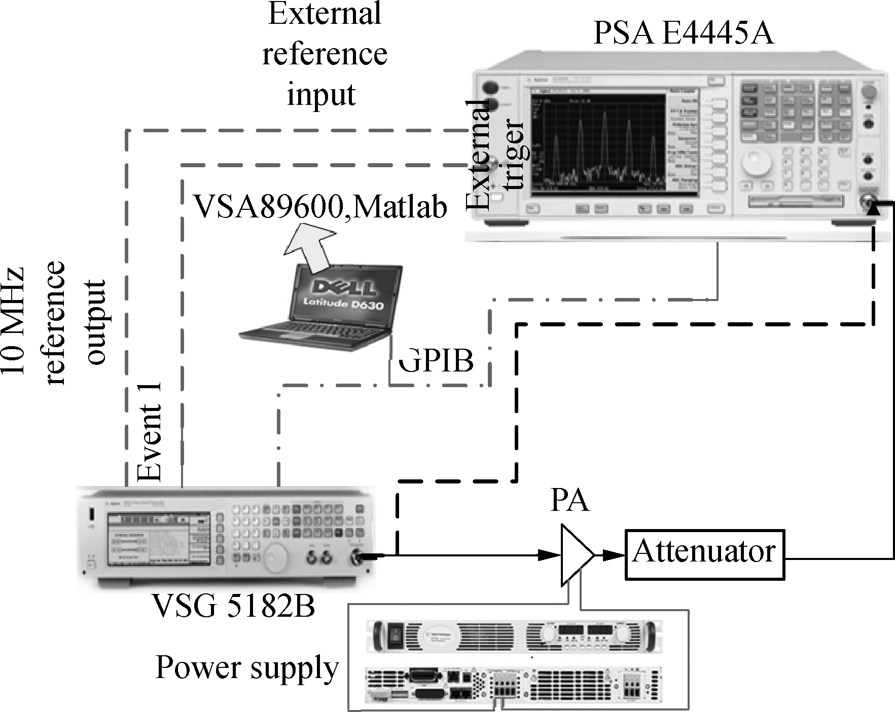
Fig.4 Block diagram of nonlinearity characterization test platform for power amplifiers
A 51 dBm peak power BPA is used in this work for modeling and linearizing validation measurement. It is a three-stage BPA applied to LTE wireless communication transmitters in the 1 880 to 1 980 MHz frequency band.
A 25-MHz mixed signal with a center frequency of 1 930 MHz is used as the test signal. It contains two carriers, namely, the 1001-CDMA2000 signal and the 1-WCDMA signal. The center frequencies of these two carriers are 1 920 and 1 940 MHz. Its peak to the average power ratio (PAPR) is 8.5. The AM/AM and AM/PM characteristics of the BPA with an average input power of -7.5 dBm is shown in Fig.5. The corresponding average output power of the BPA is 42.3; the gain of BPA is 49.8 dB, and the BPA shows strong static nonlinearity and memory effect.
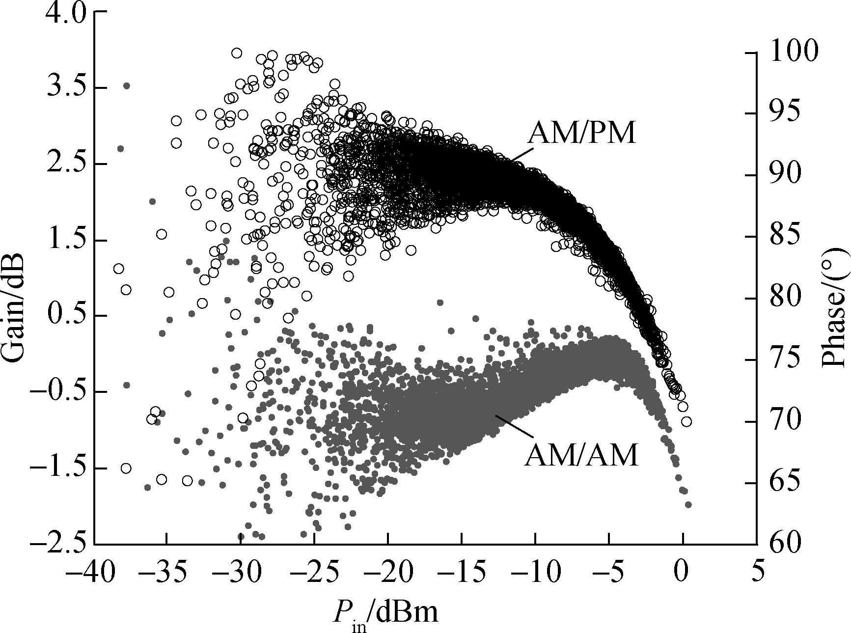
Fig.5 Measured AM/AM and AM/PM characteristics of BPA under application of -7.5 dBm test signals
1.3 Training and performance assessment of hybrid TDNN-based nonlinear model
The training of the real and complex-valued hybrid TDNN model involves two stages: hidden layer training and output layer training. In the first stage, the orthogonal least square (OLS) training scheme is employed as a forward regression procedure to determine the centers of the model (Ci(m)). The number of regression steps is equal to the number of hidden nodes. Then, the weight wi of the model can be obtained through singular value decomposition. After the centers and the weight of the hybrid TDNN are determined, the model is thus obtained.
Three thousand (3k) sample data from the mixed signal measurements was used to train the real and complex-valued hybrid TDNN. Another ten thousand (10k) sample data was used to test the training model.
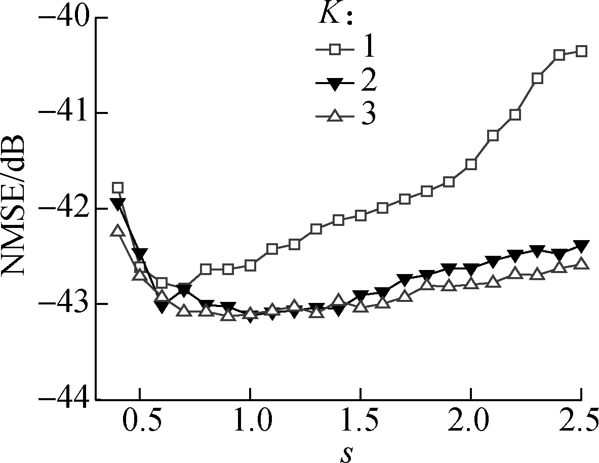
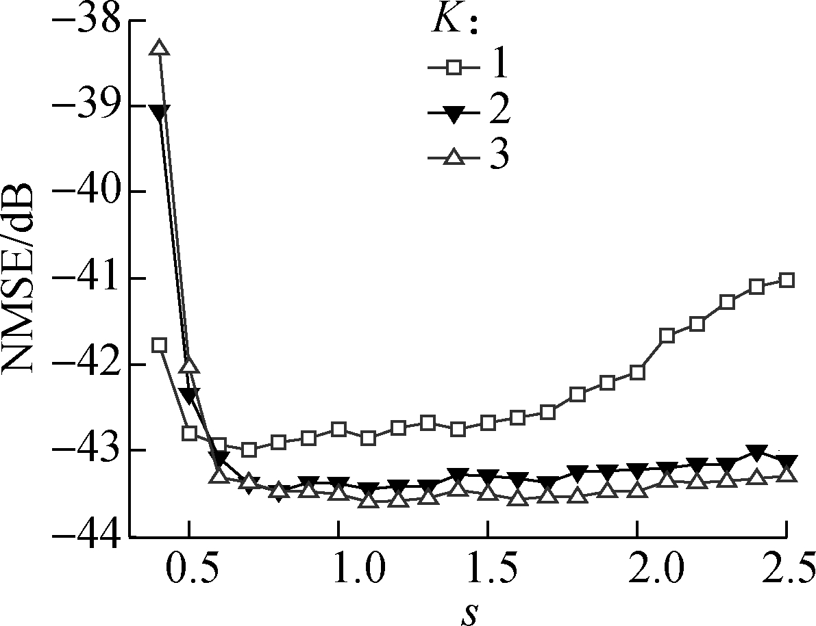
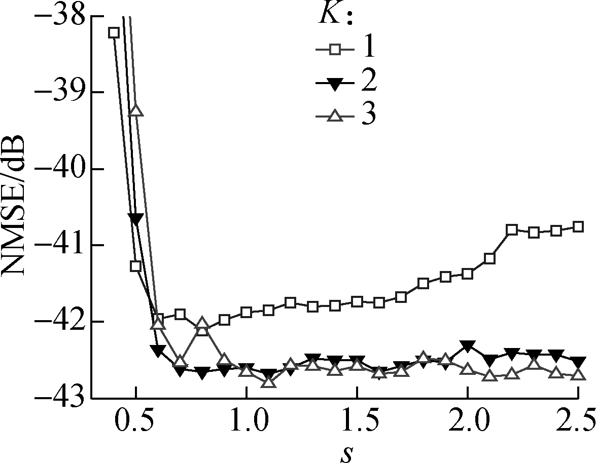
The leading memory depth M, the spread constant s, and the maximum order K of the real and complex-valued hybrid TDNN model were selected by a comparative analysis procedure, which is a NMSE-based optimization process. The NMSEs of the model were compared for different leading memory depths M from 0 to 2 in steps of 1, spread constants s from 0.4 to 2.5 in steps of 0.1, and K from 1 to 3 in steps of 1. To ensure that the real and complex-valued hybrid TDNN uses the same number of input data for the same K, the aligned memory depth M1=…Mk…=MK+1 and M1+M=3 are set up.
When the BPA with 51-dBm peak power is driven by a 25-MHz mixed signal with an average input power of -7.5 dBm, the NMSE performance in the comparative analysis is shown in Figs.6(a), (b) and (c) for 260 nodes. Here, s varies from 0.4 to 2.5 in steps of 0.1; and the leading memory depth is M=0, 1, and 2. The NMSE performance of the real and complex-valued hybrid TDNN model is compared by different K and the same leading memory depth M.
(a)
(b)
(c)
Fig.6 The NMSE performance of real and complex-valued hybrid TDNN model for (a) M=0, (b) M=1, (c) M=2
From Figs.6(a), (b) and (c), the higher the orderK of the real and complex-valued hybrid TDNN model, the higher the modeling accuracy for different s and leading memory depths M. When K=3, the NMSE of the real and complex-valued hybrid TDNN model is the minimum compared with those when K=1 and 2. However, it is 0.1 dB better, and it converges slower than that when K=2. Therefore, in this study, we select K=2.
For the same order K of the real and complex-valued hybrid TDNN model, the leading memory depth M and s have certain impacts on model accuracy. When the leading memory depth M=1, the NMSE of the real and complex-valued hybrid TDNN model has optimal performance compared with those when M=0 and 2. This is because the leading memory depth M and the aligned memory depths M1=…Mk…=MK+1 are considered, and the aligned memory depth is greater than the leading memory depth. Meanwhile, the real and complex-valued hybrid TDNN model has the same number of input data at M=0, 1, and 2 for the same K and the same number of nodes, so the real and complex-valued hybrid TDNN model has the same computational complexity. Thus, we select M=1.
From Fig.6(c), the spread constant of 0.8 is selected for K=2 since this value results in optimal modeling accuracy.
In summary, the real and complex-valued hybrid TDNN model has optimal NMSE performance, computational complexity, and modeling accuracy for M=1, K=2, and s=0.8.
In order to determine the optimal number of hidden nodes L in the proposed model and to demonstrate its merits based on the above parameters, the above four models, namely, real and complex-valued hybrid TDNN, real-valued TDNN, real-valued NN and complex-valued TDNN, are compared in terms of NMSE by varying the number of nodes from 80 to 320 in steps of 60. The NMSE performance of these four models is shown in Fig.7, where Fig.7 corresponds to the input power of -7.5 dBm. In the experiment, for the real-valued TDNN and the complex-valued TDNN models, the memory depth is 3.
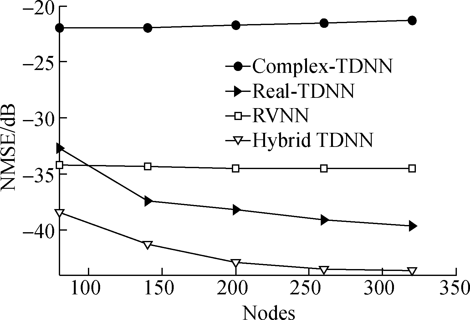
Fig.7 Performances of different models in terms of NMSE
Meanwhile, the real and complex-valued hybrid TDNN model shows significant improvement compared with the real-valued TDNN, real-valued NN, and complex-valued TDNN models in terms of modeling accuracy for BPA nonlinearity with an average input power of -7.5 dBm. Especially, for the strong nonlinearity of the BPA, the NMSE of the real and complex-valued hybrid TDNN model improves 5 dB compared to the real-valued TDNN model for 200 nodes. Therefore, the optimal number of nodes is set to be 200 to ensure that the real and complex-valued hybrid TDNN and the real-valued TDNN models have optimal modeling accuracy and computational complexity. In conclusion, the real and complex-valued hybrid TDNN model has a greater advantage over other NN models in modeling the memory effect and the static nonlinearity of the PA.
In order to further demonstrate the merits of the proposed model based on the above parameters, three other models, namely, GMP, MP, and rational function-based (RFM) model[14], were compared with the real and complex-valued hybrid TDNN model in terms of NMSE and degree of dispersion Δ. The degree of dispersion is used to illustrate the degree of divergence of the model coefficients, which is defined as the ratio of the maximum and the minimum of the coefficient modulus.
The degree of dispersion is defined as follows:
(10)
where B is the vector of the model coefficient.
When p is even, the RFM model[14] can be written as
![]()
![]()
(11)
The NMSE values of three other models are compared in Fig.8 for the BPA with the mixed test signals described in this work, where La=Lb=Lc=4, Mb=Mc=1, and Ka-1=Kb=Kc∈[2,3,4,5,6,7] for GMP1, M=4 and K-1∈[2,3,4,5,7] for MP1, La=Lb=Lc=5, Mb=Mc=1, and Ka-1=Kb=Kc∈[2,3,4,5,6,7] for GMP2, M=5 and K-1∈[2,3,4,5,7] for MP2. For the RFM model, MN=MD=4, and PN=PD∈[2,3,4,5,6,7] is for RFM1, MN=MD=5, and PN=PD∈[2,3,4,5,6,7] is for RFM2. In the compromise selection process between the NMSE and the number of coefficients, La=Lb=Lc=4, Mb=Mc=1, and Ka-1=Kb=Kc=4 are selected for the GMP model. M=5 and K=5 are selected for the MP model. However, MN=MD=5 and PN=PD= 2 are selected for the RFM model. The real and complex-valued hybrid TDNN model has 200 nodes, K=2, M=1, and s=1.5. The NMSE and the degree of dispersion Δ of these models for these parameters are compared in Tab.1.
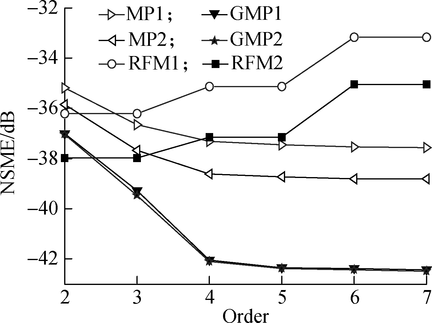
Fig.8 The NMSE values of different models
From Tab.1, we can easily conclude that the real and complex-valued hybrid TDNN and the GMP models are considerably better than the MP and the RFM models in terms of modeling strong nonlinearity of power amplifiers for broadband applications. At the same time, the NMSE of the real and complex-valued hybrid TDNN model is 0.6 dB better than that of the GMP model, and also the former has a lower degree of dispersion than the latter. At the same time, the NMSE of the real and complex-valued hybrid TDNN model is 5 dB better than that of the MP and the RFM models, and its degree of dispersion is close to that of the RFM model; the degree of dispersion of the RFM model is smaller than those of the other models.
Tab.1 NMSE and degree of dispersion Δ of different models

ModelNMSE/dBΔHybrid TDNN-42.912 5660.276 1GMP-42.367 251 617MP-38.746 58 082.5RFM-37.975 9398.855 6
2 Measurement Results of Hybrid TDNN-Based Digital Predistortion
In order to take real and complex-valued hybrid TDNN predistorters into linearization applications, the input baseband complex data of the predistorter is saved in the PC as a text file. This baseband complex data is generated by the ADS in a given period of time, so that the lead and the past inputs of the predistorter are known.
The real and complex-valued hybrid TDNN model is used to design a digital predistorter. First, the output baseband complex sample data is time-aligned and normalized with the input baseband complex sample data. Next, 3 000 output baseband sample data and 3 000 input baseband sample data are used to train the reverse model to extract the predistorter coefficients. Then, the input baseband complex data is predistorted, and the predistorted data of the predistorter is converted into the analog domain and up-converted into the respective given carrier frequencies, and then finally fed to the PA. The predistorter is then implemented in Matlab, and predistorted signals are used to linearize the BPA. This amounts to linearization of the mixed predistorted signals at an input power of -9 dBm, equal to about 1.5 dB of back-off for the input power of -7.5 dBm.
Fig.9 shows the power spectrum density (PSD) of the BPA for various predistorters. Each graph shows the BPA output spectrum with and without DPD correction. In Fig.9, the real and complex-valued hybrid TDNN and the real-valued TDNN models have the above-mentioned optimal number of nodes. At the same time, in the case of the real and complex-valued hybrid TDNN model, M=1, K=2, M1=…Mk…=MK+1=2, and s=0.8. The memory depth of the real-valued TDNN model is 3. In addition, the parameters of the GMP and the MP models are the same as those used in Section 1.3.
It is clear from Fig.9 that the performance of the real and complex-valued hybrid TDNN predistorter is significantly better than that of the optimal real-valued TDNN model and the MP model in terms of suppressing spectral regrowth when the BPA has a strong memory effect and static nonlinearity. In addition, the real and complex-valued hybrid TDNN model and the GMP model have similar linearization capabilities. However, the real and complex-valued hybrid TDNN model has better numerical stability.
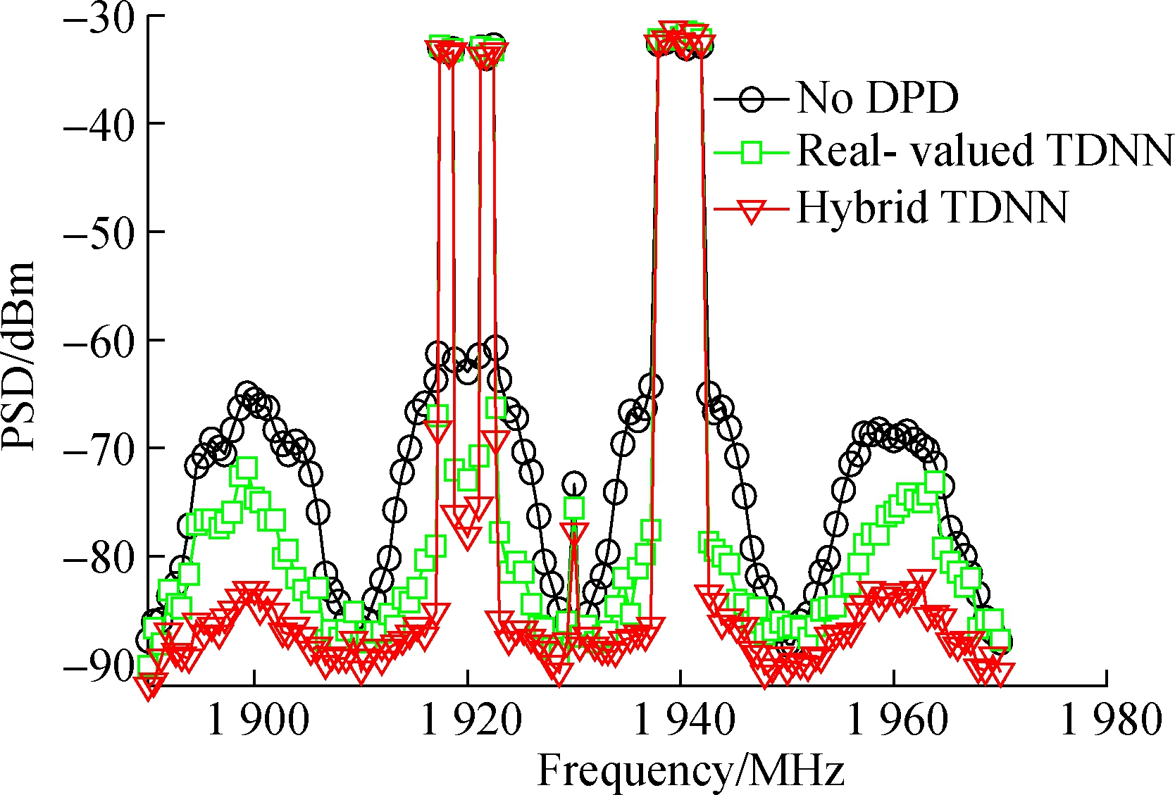
(a)
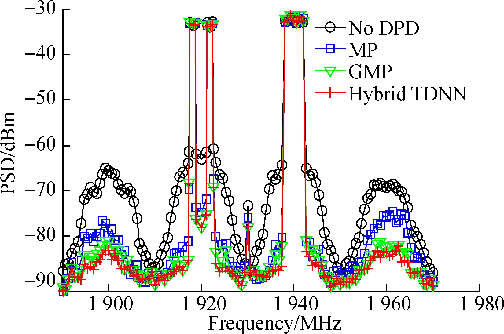
(d)
Fig.9 Comparison of output spectra for BPA linearized using different digital predistorters. (a) Of real-valued TDNN and hybrid TDNN; (b)Of MP, GMP and hybrid TDNN
From the above, the optimal NMSE, computational complexity, and linearization capability of the real and complex-valued hybrid TDNN model are determined by the selection of the aligned memory depth, leading memory depth, spread constant, and model order.
3 Conclusion
In this paper, a real and complex-valued hybrid TDNN model is proposed, which can learn and predict the strongly dynamic nonlinearity of a BPA. In addition, a predistortion technique based on the hybrid TDNN model is presented for linearizing BPA.
Three other neural networks and three other polynomial models are selected for comparison with the hybrid TDNN model, namely, the real-valued TDNN, real-valued NN, complex-valued TDNN, MP, RFM, and GMP. Through the comparative study, the optimal numbers of nodes of the hybrid TDNN and the real-valued TDNN are obtained for a real BPA driven by a -7.5 dBm mixed signal. Indeed, the optimal hybrid TDNN model leads to a nearly 5 dB improvement in the NMSE compared with the optimal real-valued TDNN model. At the same time, compared with the MP and GMP models, the optimal hybrid TDNN model is highly effective, leading to an improvement of 5 dB and 1.4 dB in the NMSE, respectively.
The linearization capability of the hybrid TDNN predistorter has been validated for a real BPA excited by mixed signals. The measurement results confirm that the optimal hybrid TDNN model significantly improves the suppression of spectral regrowth than the optimal real-valued TDNN and MP model in terms of the memory effect and static nonlinearity. In addition, the hybrid TDNN and GMP models have similar linearization capabilities, whereas the hybrid TDNN model has better numerical stability.
[1]Iqdour R, Jabrane Y. High power amplifier predistorter based on fuzzy wavelet neural networks for WiMAX signals [J]. Contemporary Engineering Sciences, 2017, 10:243-251. DOI:10.12988/ces.2017.611183.
[2]Chen S, Hong X, Khalaf E, et al. Adaptive B-spline neural network based nonlinear equalization for high-order QAM systems with nonlinear transmit high power amplifier [J]. Digital Signal Processing, 2015, 40:238-249. DOI:10.1016/j.dsp.2015.02.006.
[3]Narendra K S, Parthasarathy K. Identification and control of dynamical systems using neural networks [J]. IEEE Transactions on Neural Networks and Learning Systems, 1990, 1(1):4-27. DOI:10.1109/72.80202.
[4]Ibnkahla M, Sombrin J, Castanie F, et al. Neural networks for modeling nonlinear memoryless communication channels [J]. IEEE Transactions on Communications, 1997, 45(7):768-771. DOI:10.1109/26.602580.
[5]Zhang C, Yan S X,Zhang Q J, et al. Behavioral modeling of power amplifier with long term memory effects using recurrent neural networks[C]//2013 IEEE International Wireless Symposium (IWS). Beijing, China, 2013. DOI: 10.1109/IEEE-IWS.2013.6616831.
[6]Li M, He S, Li X. Complex radial basis function networks trained by QR-decomposition recursive least square algorithms applied in behavioral modeling of nonlinear power amplifiers [J]. International Journal of RF and Microwave Computer-Aided Engineering, 2009, 19(6):634-646. DOI:10.1002/mmce.20387.
[7]Rawat M, Rawat K, Ghannouchi F M. Adaptive digital predistortion of wireless power amplifiers/transmitters using dynamic real-valued focused time-delay line neural networks [J]. IEEE Transactions on Microwave Theory and Techniques, 2010, 58(1): 95-104. DOI:10.1109/tmtt.2009.2036334.
[8]Liu TJ, Hui M, Ye Y, et al. Linearizer for Doherty power amplifiers based on augmented general fractional order memory polynomial [J]. Journal of Sichuan University: Engineering Science Edition, 2014, 46(1):107-113. (in Chinese)
[9]Ibukahla M, Sombria J, Castanie F, et al. Neural networks for modeling nonlinear memoryless communication channels [J]. IEEE Transactions on Communications, 1997, 45(7):768-771. DOI:10.1109/26.602580.
[10]Ma Y L,Yamao Y, Akaiwa Y, et al. Wideband digital predistortion using spectral extrapolation of band-limited feedback signal [J]. IEEE Transactions on Circuits and Systems I: Regular Papers, 2014, 61(7):2088-2097. DOI:10.1109/tcsi.2013.2295897.
[11]Xu G M, Liu T J, Ye Y, et al. Generalized two-box cascaded nonlinear behavioral model for radio frequency power amplifiers with strong memory effects [J]. IEEE Transactions on Microwave Theory and Techniques, 2014, 62(12):2888-2899. DOI:10.1109/tmtt.2014.2365459.
[12]Hui M, Liu T J, Zhang M. Augmented radial basis function neural network predistorter for linearisation of wideband power amplifiers [J]. Electronic Letters, 2014, 50(12):877-879. DOI:10.1049/el.2014.0667.
[13]Morgan D R, Ma Z, Kim J, et al. A generalized memory polynomial model for digital predistortion of RF power amplifiers [J]. IEEE Transactions on Signal Processing, 2006, 54(10):3852-3860. DOI:10.1109/tsp.2006.879264.
[14]Cunha T M, Lavrador P M, Lima E G, et al. Rational function-based model with memory for power amplifier behavioral modeling [C]// 2011 Workshop on Integrated Nonlinear Microwave and Millimetre-Wave Circuits(INMMIC). Vienna, Austria, 2011. DOI:10.1109/inmmic. 2011.5773328.