Time-load history can be obtained using the long-term measurements. However, the extreme load is difficult to estimate during design life. The extreme value theory is a common method to determine the extreme load. In this theory, two sets of extreme loads above the high threshold and under the low threshold are extracted. Then, some statistical models are selected to reconstruct two new sets of new extreme loads and replace the old ones randomly[1-13]. Too low or too high extreme thresholds will result in high estimation variances[4-5]. To find the proper threshold, researchers[6-7] proposed many effective methods[8-10]. Thompson et al.[11] created a method to check a series of gradually increasing thresholds until one passed the null hypothesis Pearson normality test. Fukutome et al.[12]presented an automated procedure for the peak-over-threshold(POT) method and used it to provide a climatology of extreme hourly precipitation.
However, there are irrational and uncertain factors in common threshold selection methods.First, due to different comprehensions of approximate linearity, the result of the graphical method varies from person to person. Secondly, the corresponding threshold cannot avoid the problem of shape parametric sensitivity of the exceedance function. Thirdly, The kurtosis method selects thresholds by deleting the sample points of load data. However, this load data is most likely to have a direct correlation with the extreme load. The bootstrapping technology (BT) proposed in this paper realizes automatic processing by computer and avoids the effect of the human factor. In addition, it can effectively avoid the fluctuation of the shape parameter of the exceedance function and solve the problem of insufficient exceedances.
1 Common Methods
The graphical approach is used to plot the mean excess function (MEF) curve of the sample. The approximate linear zone from the right part of the curve is selected. The minimum threshold corresponding to this zone is regarded as the optimal one.
The mean excess function is defined as

(1)
where u is the threshold; Nu is the amount of sample load, which is greater than u.
The basic principle of the kurtosis method is that the intersection of normal distribution and skewness distribution is the optimal threshold. The kurtosis of the load sample data is calculated by
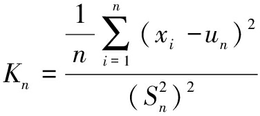
(2)
where ![]() is the sample variance,
is the sample variance, ![]() un is the mean of the sample data,
un is the mean of the sample data, ![]() When the sample kurtosis is less than 3, the smallest value xi is the optimal threshold.
When the sample kurtosis is less than 3, the smallest value xi is the optimal threshold.
2 Bootstrapping Technology
Mooney et al.[13] described the accuracy and stability characteristics of the data. Bias underestimates or overestimates the true value and describes the matching precision and quality[13]. In load sample statistical properties, the greater the bias, the less the variance. The mean squared error (MSE) can evaluate any threshold based on the estimators of variance and bias. The optimal threshold is found by minimizing an approximate expression of MSE. The MSE is calculated by a given set of data as
MSE(X)=bias2(X)+var(X)
(3)
The bias of exceedance is closely related to the population mean. However, the real mean value cannot be obtained by just enlarging the sample size. If we define the estimated value of the small load sample as the population mean, a large error will emerge. The estimation of population parameters requires new paths.
Bootstrapping[14] is used to determine the variance and the bias associated with estimation. Suppose that data set y is a random sample of exceedance, and the distribution form of F is unknown aforehand. θ=θ(F) is one of the true distribution parameters of F, and φ=φ(Fn) (Fn is the specific type of distribution function) is the corresponding estimated value of θ. The deviation between the estimated value and true value is then calculated by
Tn=φ(Fn)-θ(F)
(4)
Each exceedance will produce several bootstrapping sample estimators, which differ from those of the original exceedance sample. Caers and Maes[15] revealed that the distribution characteristic of the bootstrapping sample is equivalent to that of the population sample.
The calculation process of Tn is shown in Fig.1 (The variables with “*” are the bootstrapping estimators), and the detailed process is summarized as follows:
1) Determine the threshold interval [umin, umax] and growth pace Δu.
2) For each of the given threshold ui, the exceedance samples χi of load data are available. To ensure the reliability and stability of parameter model, the exceedance sample should contain at least 25 pieces of data.
3) Calculate the mean ![]() of the exceedance sample (original sample) data.
of the exceedance sample (original sample) data.
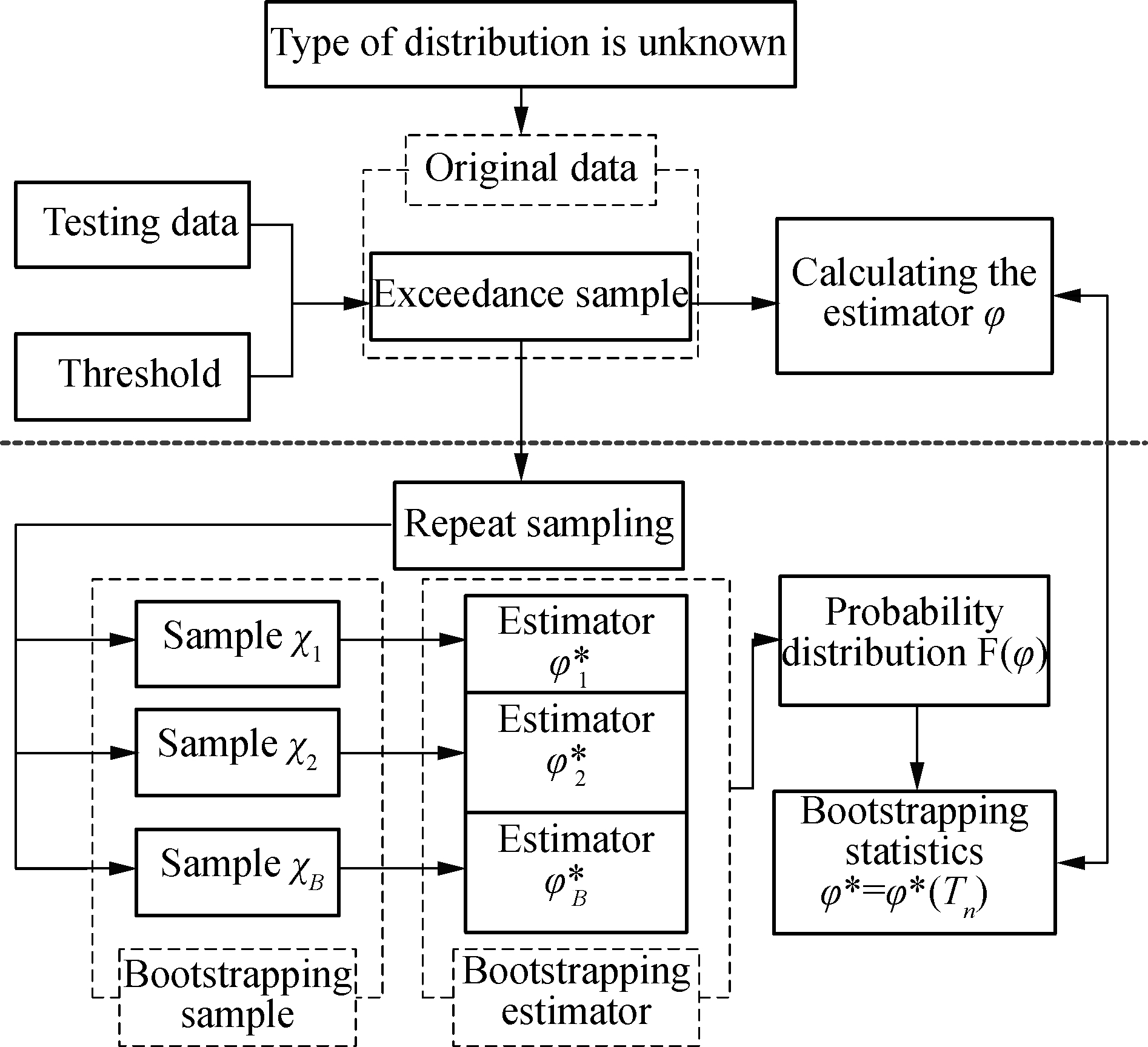
Fig.1 Calculation flow chart for Tn
4) Set the bootstrapping sampling frequency, b=1,2,…,B. When B=200, the estimated bias and variance of a data set can generally meet the accuracy requirement.Bootstrapping sampling with the replacement from sample χi is conducted, so that ![]() (the b-th sample of the i-th interval) can be obtained. The mean of the b-th load sample
(the b-th sample of the i-th interval) can be obtained. The mean of the b-th load sample ![]() is calculated. The average of all the sample mean
is calculated. The average of all the sample mean ![]() is calculated.
is calculated.
5) Calculate the estimators of bias, var and MSE of the exceedance sample.
6) Record the processing results, then select the threshold ui+1, and repeat steps 3) to 5).
Using this method, bias, var and MSE are, respectively, calculated as
(5)
(6)
(7)
where φ(b) is the estimator of parameter θ corresponding to the b-th sample.
3 Goodness of Fit Test
3.1 Graphical method
In statistics, the quantile-quantile plot (QQ-plot) is a convenient visual tool to examine whether a sample comes from a specific distribution or not. Specifically, the quantiles of an empirical distribution are plotted against the quantiles of a hypothesized distribution. If the sample comes from the hypothesized distribution, the QQ-plot is linear.
3.2 Numerical method
The average deviation of the probability density function is used to describe the average of distribution deviation absolute value on all sample points of measured data and the theoretical data model of the probability density function, which is defined as
(8)
where f(x) is the probability density function of the measured data, and g(x) is the probability density function of the theoretical distribution function.
3.3 Parametric sensitivity analysis method
The generalized Pareto distribution (GPD) model has two parameters. One is the shape parameter, and the other one is the scale parameter. If the value of the shape parameter estimated according to the exceedance does not change obviously, the exceedances which are decided by the selected threshold obey the generalized Pareto distribution[16].
4 Case Study
To verify the method proposed in this paper, the testing sample data of pump 1 outlet pressure of the excavator under the working condition of small stones, as shown in Fig.2, is given to illustrate the detailed process of determining the optimal threshold.
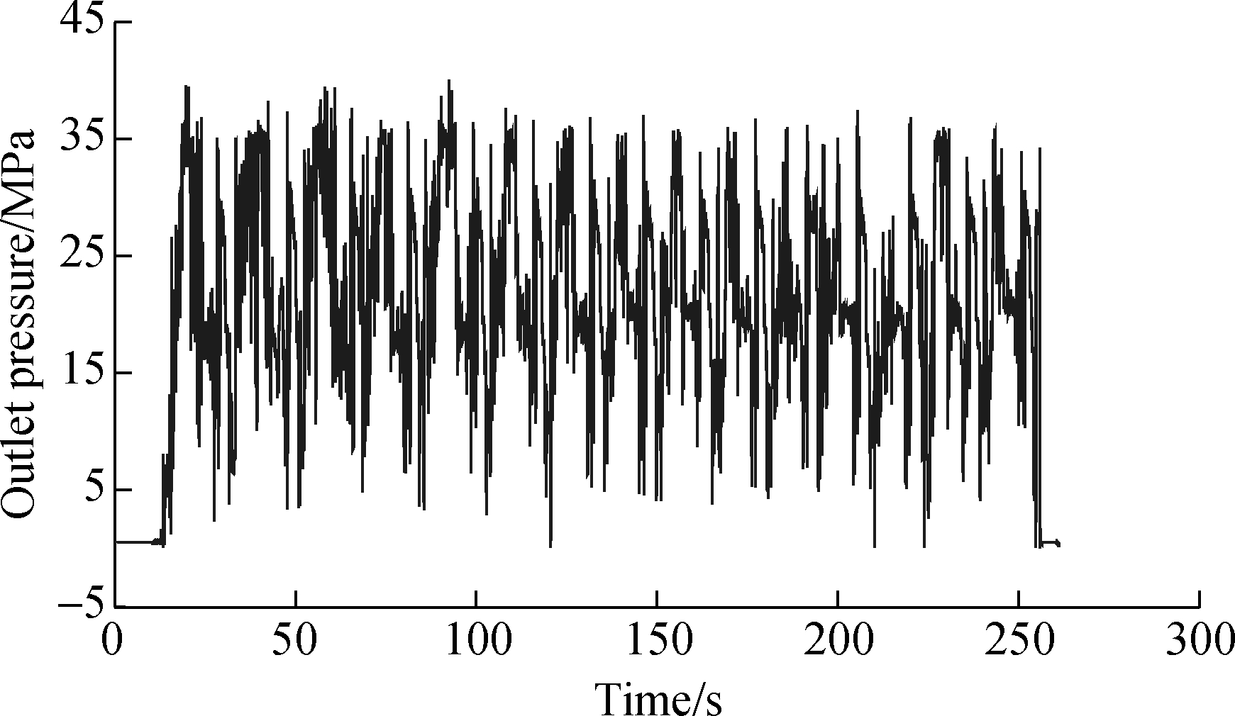
Fig.2 Data of pump outlet pressure of excavator
4.1 Calculation of threshold
In order to verify the validity and rationality of the method proposed in this paper, three methods are used on the same data.
First, based on the the sample data and formula (2), the optimal threshold is 201 according to the kurtosis method.
Secondly,based on the sample data, Fig.3 can be obtained by applying the above MEF method. The minimum e(u) of the section, which is close to the graphic right and approximately linear, is the optimal threshold. It can be seen that, when the threshold is between 305 and 340, the curve is linear. When the threshold is larger than 340, the curve is nonlinear. Therefore, the optimal threshold is 306.32.
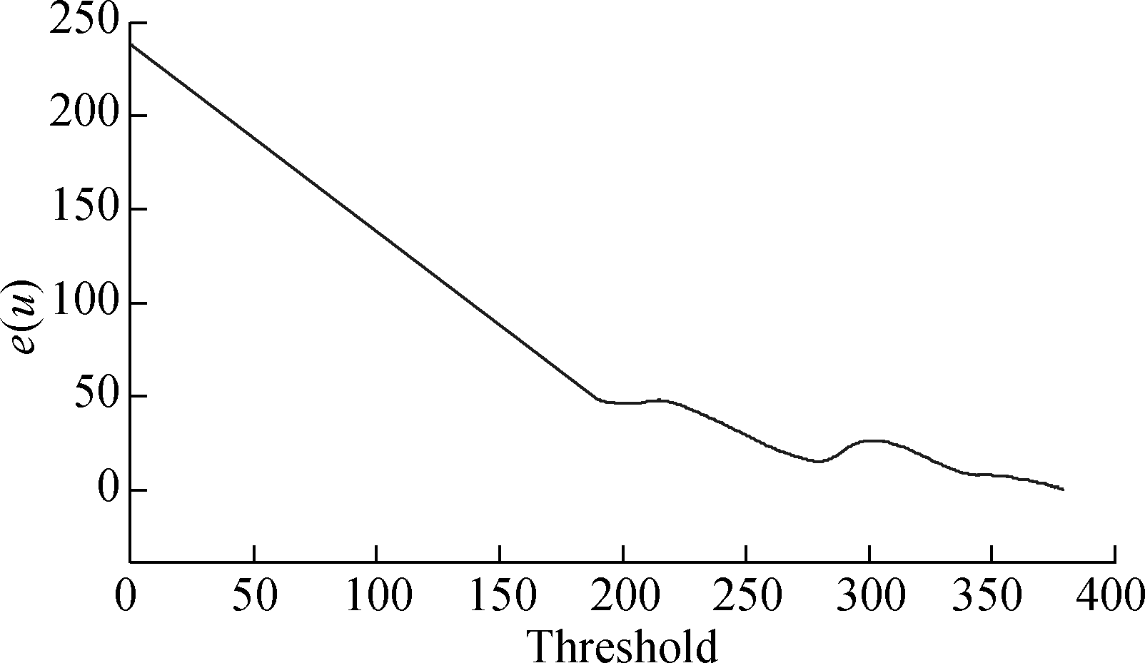
Fig.3 Optimal threshold obtained by the MEF method
(a)
(b)

(c)
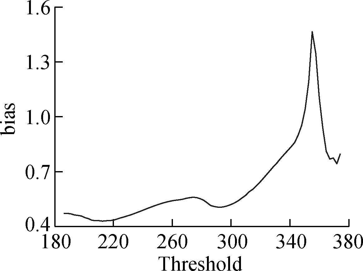
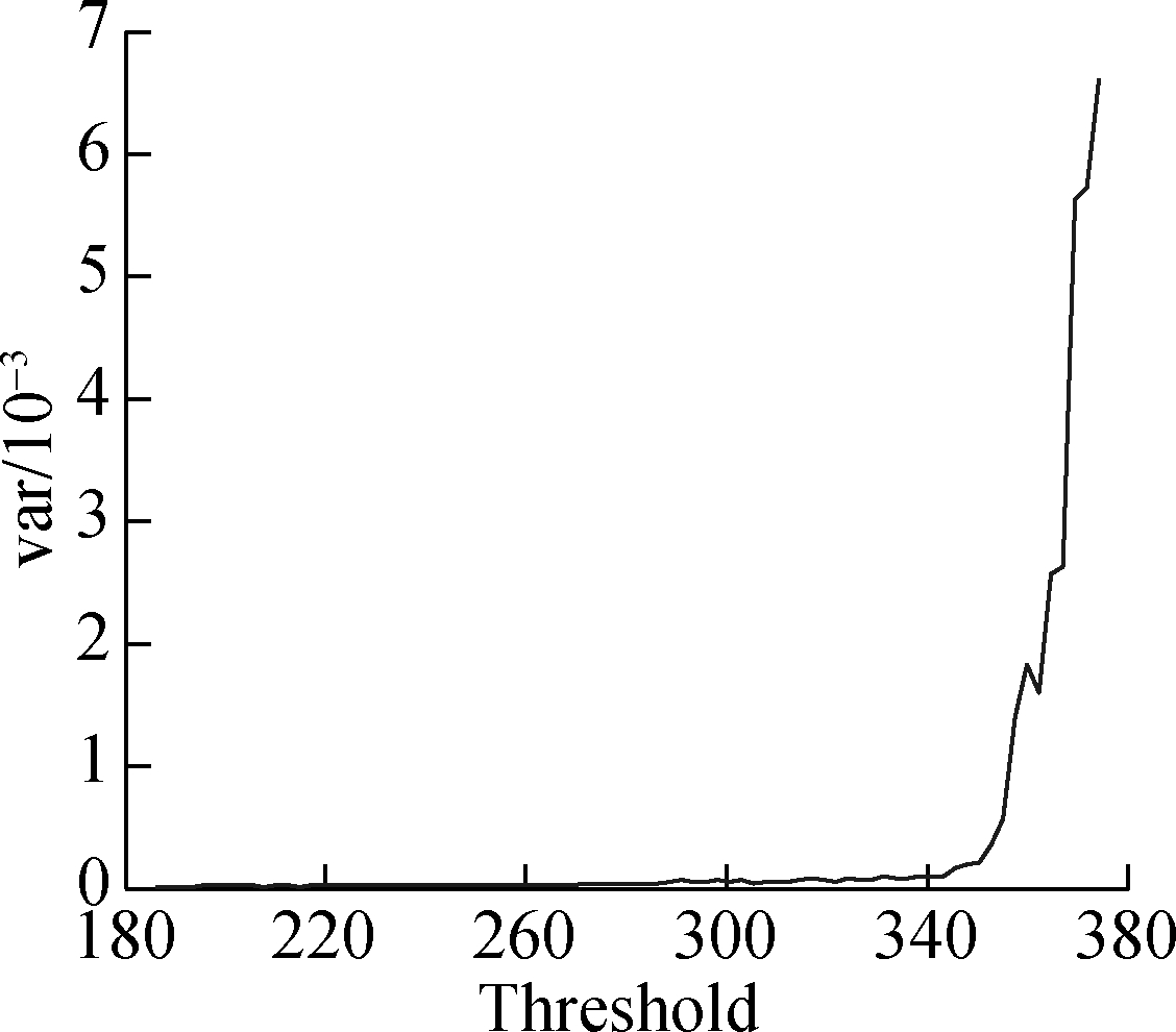
Fig.4 Optimal threshold obtained by the MSE method based on automated sampling. (a) Bias estimation; (b) Variance estimation; (c) MSE estimation
Thirdly, Fig.4 can be obtained by the MSE method based on automated sampling. The threshold when the MSE is the minimum is the best threshold. By viewing the data results, the MSE is the minimum when the threshold is 212.16. Therefore, the optimal threshold is 212.16.
4.2 Fitting test of threshold
4.2.1 Graphical method
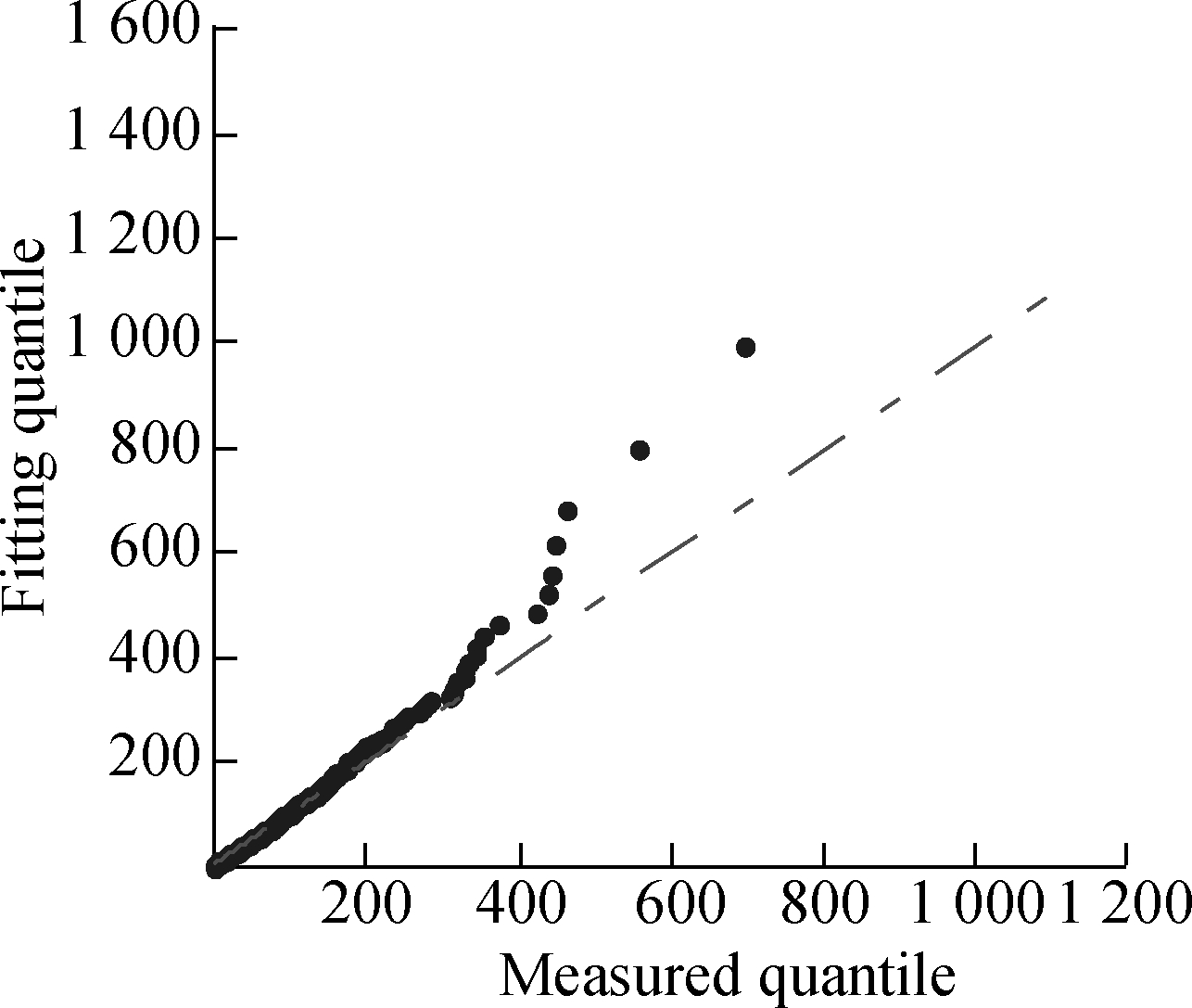
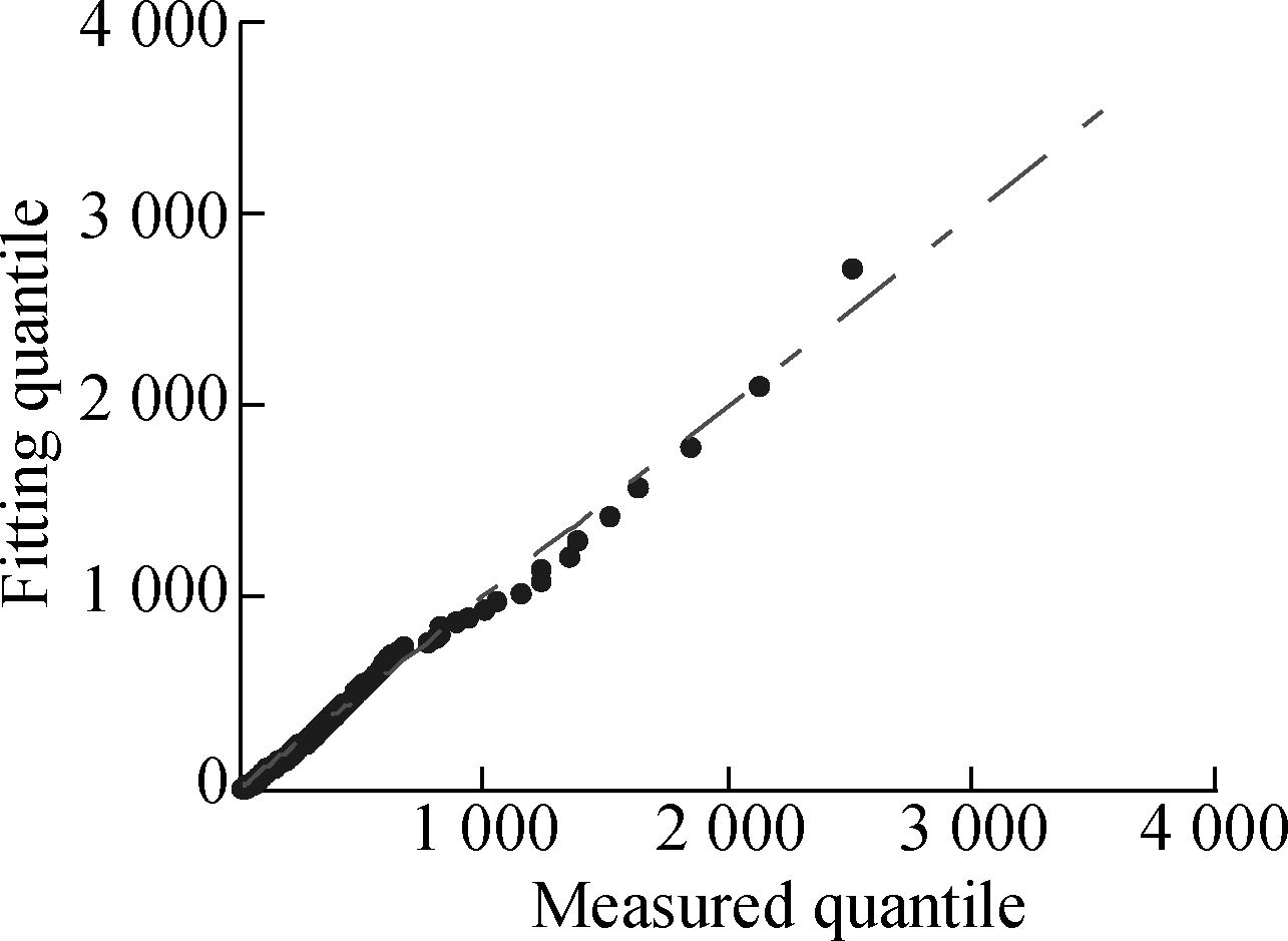
As shown in Fig.5, QQ-plots show the relationship between the empirical data and the GPD. The plots of Figs.5(a) and (b) show that points are not on the line in the large load region. The plot of Fig.5(c) is similar to a straight line. Therefore, it is clear that Fig.5(c) has a better fitting result. The threshold ω, which is calculated by BT, is more accurate.

(a)
(b)
(c)
Fig.5 QQ-plot under different thresholds. (a) ω=201; (b) ω=306.32; (c) ω=212.16
4.2.2 Numerical method
According to the numerical method, the results are presented in Tab.1. Compared to the kurtosis method and the MEF method, the average deviation of the probability density function of exceedances decided by BT reduces 38.52% and 29.25%, respectively.
Tab.1 Comparisons of optimal threshold and average deviation based on different methods

MethodKurtosis methodMEF method BT methodOptimal threshold201.00306.32212.16Average deviation of proba-bility density function0.012 20.010 60.007 5
4.2.3 Parametric sensitivity analysis
In Fig.6, the solid line represents the changes of shape parameter corresponding to the exceedance of different thresholds. The dashed lines represent a 95% confidence interval(CI). For each threshold, the probability of its shape parameter falling between the two dashed lines is 95%. It can be seen clearly that the shape parameters corresponding to thresholds in the vicinity of 212.16 are essentially constant. However, the shape parameters corresponding to thresholds in the vicinity of 201.00 and 306.32 show obvious variation.
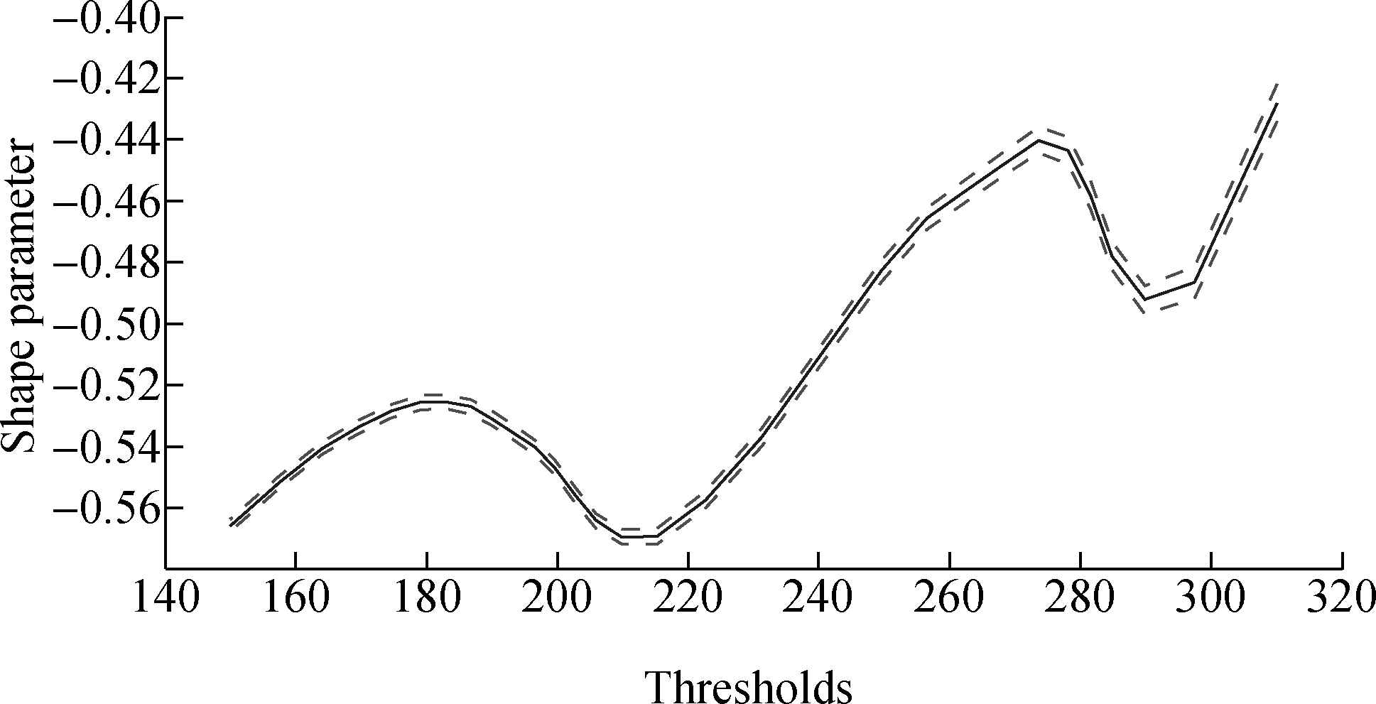
Fig.6 Shape parameters of exceedances
5 Conclusion
The threshold obtained by the BT method is more reasonable and the exceedances are better for fitting the GPD function. Also, the shape parameters near the threshold is more stable. Compared to the kurtosis method and the MEF method, the average deviation of the probability density function of exceedances decided by BT reduces 38.52% and 29.25%, respectively. In addition, the BT method enlarges the original samples and avoids the randomness and poor credibility of the results, which can solve the instability of the original distribution parameters caused by insufficient exceedances .
[1]Gomes M I, Guillou A. Extreme value theory and statistics of univariate extremes: A review[J]. International Statistical Review, 2014, 83(2): 263-292. DOI:10.1111/insr.12058.
[2]Mailhot A, Lachance-Cloutier S, Talbot G, et al. Regional estimates of intense rainfall based on the peak-over-threshold (POT) approach[J]. Journal of Hydrology, 2013,476:188-199. DOI:10.1016/j.jhydrol.2012.10.036.
[3]Naess A, Haug E. Extreme value statistics of wind speed data by the POT and ACER methods[J]. Journal of Offshore Mechanics and Arctic Engineering, 2010, 132(4): 041604. DOI:10.1115/1.4001419.
[4]Bernardara P, Mazas F, Weiss J, et al. On the two step threshold selection for over-threshold modelling[C]// Proceedings of 33rd Conference on Coastal Engineering. Santander, Spain, 2012 (33):42. DOI:10.9753/icce.v33.management.42.
[5]Scarrott C J, Macdonald A. A review of extreme value threshold estimation and uncertainty quantification[J]. REVSTAT-Statistical Journal, 2012,10(1) :33-60.
[6]You Z J. Discussion of “a multi-distribution approach to pot methods for determining extreme wave heights” by Mazas and Hamm, [Coastal Engineering, 58:385-394][J]. Coastal Engineering, 2012,61:49-52. DOI:10.1016/j.coastaleng.2011.11.004.
[7]Mazas F, Hamm L. Reply to discussion by Z.J. You of “A multi-distribution approach to POT methods for determining extreme wave heights” by Mazas and Hamm[J]. Coastal Engineering, 2012,65:16-18. DOI:10.1016/j.coastaleng.2012.02.008.
[8]Mazas F, Hamm L. A multi-distribution approach to POT methods for determining extreme wave heights[J]. Coastal Engineering, 2011,58(5):385-394. DOI:10.1016/j.coastaleng.2010.12.003.
[9]Gomes M I, Figueiredo F, Martins M J, et al. Resampling methodologies and reliable tail estimation[J]. South African Statistical Journal, 2015, 49(1): 1-20.
[10]Li F, Bicknell C. A comparison of extreme wave analysis methods with 1994—2010 offshore Perth dataset[J]. Coastal Engineering, 2012,69:1-11. DOI:10.1016/j.coastaleng.2012.05.006.
[11]Thompson P, Cai Y, Reeve D, et al. Automated threshold selection methods for extreme wave analysis[J]. Coastal Engineering, 2009,56(10) :1013-1021. DOI:10.1016/j.coastaleng.2009.06.003.
[12]Fukutome S, Liniger M A, Sueveges M. Automatic threshold and run parameter selection: a climatology for extreme hourly precipitation in Switzerland[J]. Theoretical and Applied Climatology, 2015,120(3/4):403-416. DOI:10.1007/s00704-014-1180-5.
[13]Mooney C Z, Duval R D. A nonparametric approach to statistical inference[J].Technometrics, 1993,36(4):435-436. DOI: 10.2307/1269981.
[14]Efron B, Tibshirani R J. An introduction to the bootstrap[J]. Chapman and Hall, 1993,23(2):49-54. DOI:10.1111/1467-9639.00050.
[15]Caers J, Maes M A. Identifying tails, bounds and end-points of random variables[J]. Structural Safety, 1998,20(1) :1-23. DOI:10.1016/s0167-4730(97)00036-2.
[16]Shi D J. Practical methods of extreme value statistics[M]. Tianjin: Tianjin Science and Technology Press, 2006. (in Chinese)