The lane-changing behaviors of vehicles are complex, which play a fundamental role in the microscopic traffic flow theory. According to the intention of lane change, lane-changing behaviors are commonly categorized into two types: mandatory lane change (MLC) and discretionary lane change (DLC). The MLC describes the behavior that the vehicle must leave the current lane while the DLC is performed to improve the driving conditions. The effect of the DLC on traffic flow is scattered and global while that of the MLC is focused and local. The complete lane-changing process is composed of a lane-changing decision (LCD), lane-changing preparation (LCP) and lane-changing execution (LCE). LCD includes the following four successive decisions: Generation of the lane-changing requirement, choice of the target lane, choice of the target gap and acceptance of the target gap. The target lane is selected from the adjacent lanes and drivers seek an appropriate target gap in the target lane. According to the characteristics of driving behavior, the first two decisions have few significant effects on vehicle’s current car-following motion. After choosing a target gap, an LCP process will be executed until the target gap is acceptable for lane change. During the LCP process, especially in a congested traffic situation, the lane-changing vehicle usually has to deliberately slow down first to wait for the target gap or to speed up to squeeze into the target gap. In this process, the following putative vehicle may slow down or switch to the other lane to let the lane-changing vehicle in. Thus, a lane-changing vehicle interacts with surrounding vehicles in its current lane and target lane during the LCP process. The LCE process is the period from the time that the lane-changing vehicle accepts the target gap to the time that the lane-changing vehicle inserts itself into the target gap successfully. The LCE process occurs right after the LCP process.
LCD has been studied adequately.A comprehensive review about LCD modelling can be referred to in Refs.[1-2]. The LCD models can be classified into four groups: Rule-based models, discrete-choice models, artificial intelligence models, and incentive-based models. Rule-based models include the Gipps model[3], CORSIM model[4], SITRAS model[5], cellular automata model[6] and game theory model[7]. Discrete-choice models include Ahmed’s model[8] and Toledo et al.’s model[9]. Artificial intelligence models include the artificial neural network model[10-11] and fuzzy-logic based model[12]. Incentive-based models include MOBIL[13] and LMRS.
Recently, the research on LCE modelling has been increasing.Moridpour et al.[14] studied LCE modelling under heavy traffic conditions, and proposed the longitudinal acceleration models for both heavy vehicles and passenger cars. Papadimitriou and Tomizuka[15] proposed a polynomial model to make automated vehicles move in both longitudinal and latitudinal directions. In the manual LCE process, the lane-changing vehicle must dynamically interact with its putative leader and follower in the target lane in the longitudinal direction accompanying a lateral movement. Kou and Machemehl[16] used the angular velocity that contained the lateral motion features to build an acceleration-deceleration model for lane-changing vehicles.Wan et al.[17] introduced visual angle information to capture the vehicle interaction behavior during the LCE process. Wang et al.[18] proposed a behavioral-based general framework for the LCE model.
The drivers’ behaviors related to the LCP have been seldom paid attention to for a long time. Hidas[19]developed a new cooperative lane-changing model incorporating explicit modelling of vehicle interactions during the LCP process using intelligent agent concepts, but the model is only a concept, not yet validated by field data. Sun and Kondyli[20]quantified the vehicle interactions during the LCP process. Schakel and Knoop[21] introduced a concept of synchronized lane change which means that a potential lane-changing vehicle intends to synchronize velocity with the vehicles in the target lane. Empirical analysis based on field trajectory data was presented to support such a concept by Wan et al.[22] and Park et al.[23], but the field data was limited to the freeway merging area.
In summary,existing research about lane-changing behavior focused on LCD and LCE. Research on LCP is rare, and the research about LCP for DLC on freeways is almost ignored. Hereafter, the LCP for DLC is called discretionary lane-changing preparation (DLCP), and similarly, the LCE for DLC is called discretionary lane-changing execution (DLCE). However, the DLCP process on a freeway plays an important role in simulating and predicting the lane-changing behavior more completely and accurately. The aim of this study is to put forward two acceleration models to simulate the longitudinal driving behaviors of the lane-changing vehicle and the following putative vehicle during the DLCP process on freeway.
1 Data Description
This study used the published dataset, collected at US Highway 101(US-101) in Los Angeles, California, USA. The entire segment of US-101 is 630 m long with five freeway lanes and an auxiliary. Starting with 1, lane numbers are incremented from the left-most lane. The US-101 data was collected from 07:50 to 08:35 on June 15, 2005. The time interval for vehicle location update is 0.1 s, and each measured sample from this data set has 18 features, such as longitudinal position, lateral position, velocity, acceleration, time, vehicle class, front vehicle number, and following vehicle number. Lane 5 and 6 are excluded from the study since lane-changing behaviors in these lanes are likely affected by the on and off ramps,but not likely to be discretionary lane changes. To obtain a homogeneous model, four additional criteria are applied for the selection of the discretionary lane-changing behavior sample:
1) The lane-changing vehicles which are trucks or motorcycles are not considered.
2) The lane-changing vehicles whose interacting vehicles include trucks or motorcycles are not considered.
3) Successive lane-changing processes are not considered.
4) The failed lane-changing processes are not considered.
5) The lane-changing vehicles whose leading vehicle (in original lane) or putative leading and following vehicle (in the target lane) changes lane at the same time are not considered.
By using the above criteria, 146 discretionary lane-changing behavior samples are selected. The corresponding data set is smoothed by the locally weighted scatterplot smoother algorithm(LOWESS)[24].
2 Identification of DLCP
Fig.1 shows the layout of a lane-changing vehicle and its interacting vehicles during DLCP process, in which the lane-changing vehicle is named as a subject vehicle and marked as“SV”. Its interacting vehicles include the leading vehicle and following vehicle on the current lane as well as the putative leading vehicle and the following putative vehicle on the target lane. They are denoted as CLV, CFV, PLV and PFV, respectively, in Fig.1. The distance between SV and real CLV, CFV, PLV or PFV is beyond 135 m. If CLV (CFV, PLV or PFV) is absent within 135 m, then a corresponding virtual vehicle (CLV, CFV, PLV or PFV) is set to be located at the position where the distance to SV is 135 m. The speed of the following virtual vehicle (CFV and PFV) is set to be 0 m/s and that of leading virtual vehicle (CLV and PLV) is set to be 30 m/s. The gap between PLV and PFV is known as the target gap of subject vehicle and denoted as gT. The piece-wise line with an arrow in Fig.1 illustrates the sketch of the whole lane-changing trajectory, where the first segment represents the trajectory during the DLCP process and the second segment represents the trajectory

Fig.1 Sketch of lane-changing vehicle and its interacting vehicles’ layout during DLCP process
during the DLCE process. To systematically identify the DLCP process, the starting point and the ending point of the DLCP process should be determined.
2.1 Identification of the starting point of DLCP process
In this study, it is assumed that once SV’s DLCP behavior is initiated and PFV obtains the signal, it will start to slow down to provide a sufficient spacing with PLV for SV inserting into target lane, which is called anticipation behavior[25]. Thus, the identification of the starting point of SV’s DLCP process can be transformed into the identification of the starting point of PFV’s anticipation behavior.
So far, two ways to identify the starting point of PFV’s anticipation behavior have been presented, but both of them have their limitations in practical applications. Zheng et al.[25] used the Newell simplified car-following theory to specify the starting point of anticipation. The starting point of anticipation is identified by intersecting the theoretical time-space trajectory of the PFV with its actual trajectory before SV inserts into the target lane. The method is based on the hypothesis that the spacing-speed relationship for a given vehicle is linear before the anticipation period, which is not consistent with real data in most cases. Ghaffari et al.[26] proposed another method for the identification of the starting point of the anticipation period. In this method, the time when PFV’s acceleration reaches the maximum before SV inserts into target lane is determined as the start of anticipation behavior. In fact, this method cannot guarantee that the target gap will become more suitable for SV inserting into the target lane after the determined starting point of the anticipation period.
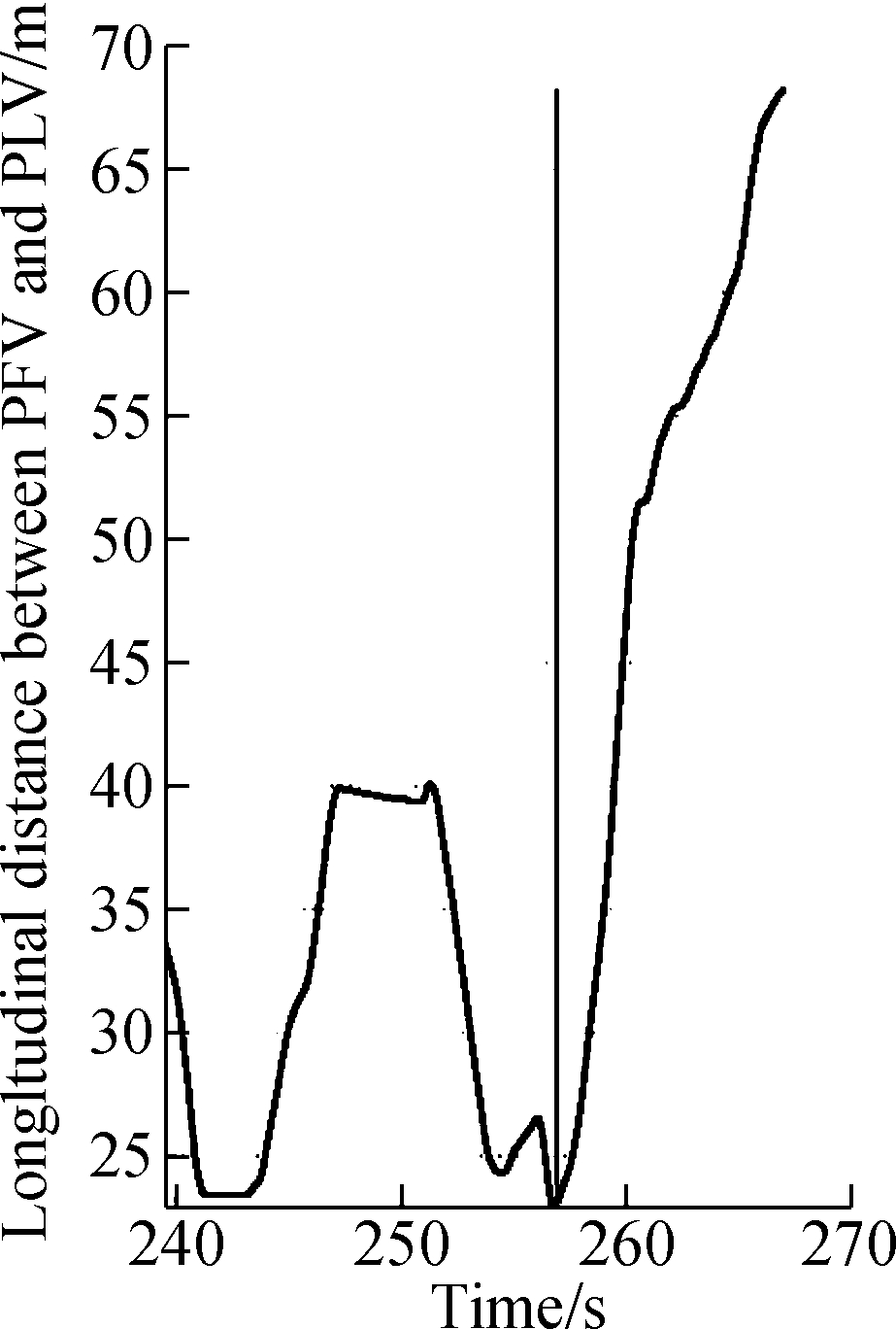
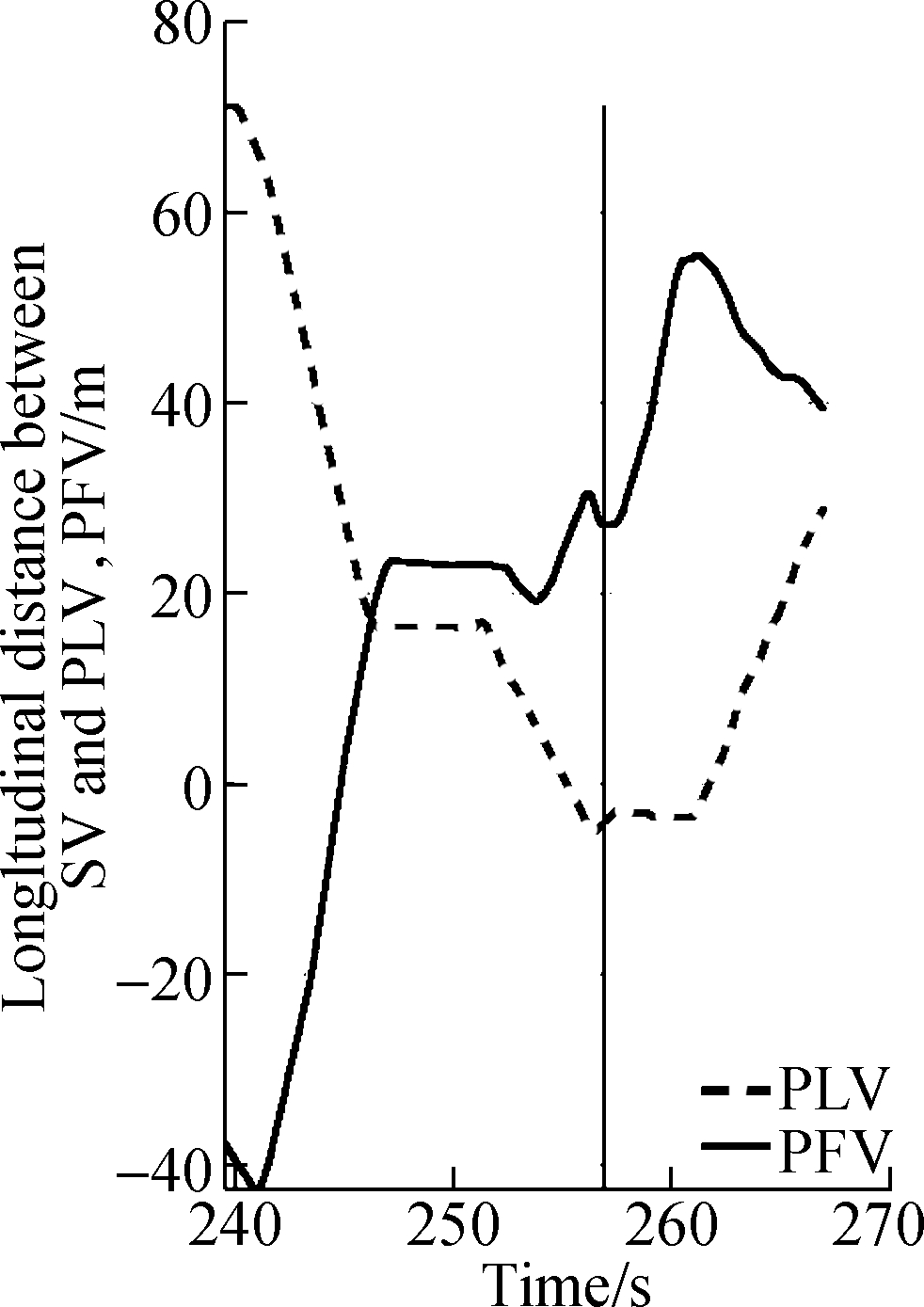
Thus, a simple but practical way is employed to identify the start of anticipation behavior by referring to the two methods mentioned above. In the new method, the time when the spacing between PFV and PLV starts to approximately enlarge significantly and continuously until SV gets into target lane, is taken as the start of the anticipation period. At the same time, another condition that the SV’s longitudinal position is close to the target gap should be satisfied. In this study, both the relative space between SV and PLV and the relative space between PFV and SV are constrained to range from -1.5 to 30 m. Taking the real SV with the vehicle ID of 410 for example,Fig.2 shows the identification results of the starting point of DLCP process. The perpendicular black line in Fig.2 represents the starting point of the anticipation period, which is captured accurately from an intuitive view.
2.2 Identification of ending point of DLCP process
DLCP occurs before DLCE, and the ending point of DLCP is the starting point of DLCE. Similarly, the identification of the ending point of SV’s DLCP process is transformed into the identification of the starting point of
(a) (b)
Fig.2 Identification of the starting point of DLCP process for SV with the vehicle ID of 410.(a) Change of longitudinal distance between PFV and PLV;(b) Change of longitudinal distance between SV and PFV, PLV
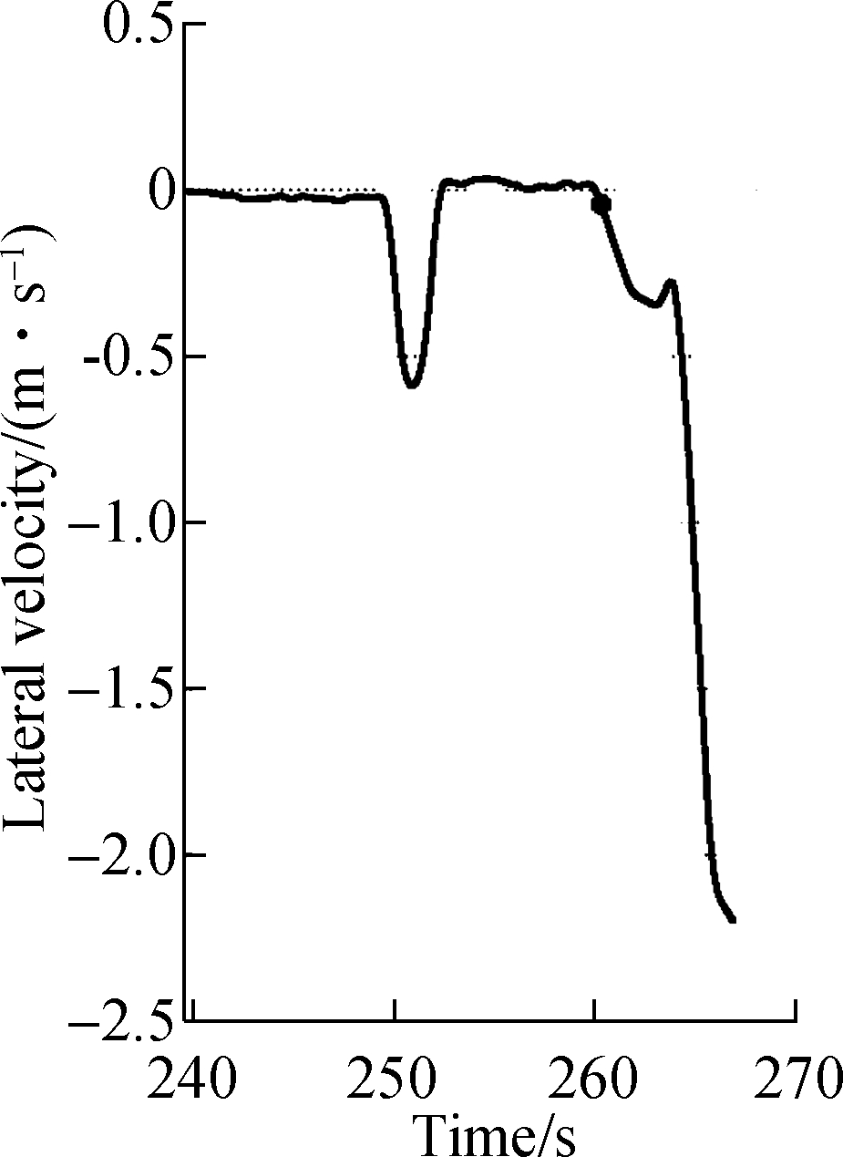
the DLCE process. The start of the lane-changing vehicle’s lateral movements toward the adjacent target lane without being interrupted is defined as the starting point of the DLCE by several researchers[14, 27]. However, this method ignores the significant change of lateral velocity when SV starts DLCE. In reality, the magnitude of lateral acceleration at this time slot often corresponds to a local maximum. Thus, in this study, when the SV moves from the original lane towards the target lane without interruption, the maximum of its lateral acceleration is denoted as the starting point of DLCE, i.e. the ending point of DLCP. Taking the real SV with the vehicle ID of 410 for example as well, the identified results of the ending point of DCLP are shown in Fig.3. The rendered black circle in Fig.3(a) and Fig.3(b)represent the identified starting point of DLCE with the traditional method and the new proposed method. In the next section, we employ the proposed method to identify the starting point of DLCE.

(a) (b)
Fig.3 Identification of ending point of DLCP process for SV with the vehicle ID of 410.(a) Change of lateral velocity of SV;(b) Change of lateral acceleration of SV
3 Acceleration Model of Lane-Changing Vehicle during the DLCP Process
By applying the identification procedure for the trajectory of DLCP process described in Section 2 on the selected NGSIM dataset, 100 groups of samples are extracted in all. The empirical observations indicate that DLCP period persists for 4 to 8 s on average with variations across sites and lanes, which suggests that the DLCP behavior is significant and should not be ignored in modelling the lane-changing behavior. The 100 selected groups of samples are randomly divided into two equal parts (50 groups each). One is employed to calibrate the proposed model and the other is applied to validate the model performance. This section focuses on modelling the longitudinal driving behavior of lane-changing vehicles during the DLCP period.
3.1 Model formulation
For the longitudinal movement during the DLCP period, SV behaves in a similar manner as it does under the normal car following situations. The difference is that SV behaves in response to CLV, PLV, and PFV simultaneously. Thus, the longitudinal governing equation of SV during DLCP period is given as
(1)
where ![]() are the longitudinal acceleration of vehicle SV at time t and
are the longitudinal acceleration of vehicle SV at time t and ![]() are the longitudinal speed of vehicle SV at time t-T, respectively;
are the longitudinal speed of vehicle SV at time t-T, respectively; ![]()
![]() and
and ![]() denotes the spatial headway with CLV, PLV and PFV of SV at t-T, respectively;
denotes the spatial headway with CLV, PLV and PFV of SV at t-T, respectively; ![]()
![]() and
and ![]() denote the relative velocity with CLV, PLV and PFV of SV at t-T, respectively.α,β,γ, ρ, ω, δ, and τ are the sensitivities of drivers; T represents the driver reaction time.
denote the relative velocity with CLV, PLV and PFV of SV at t-T, respectively.α,β,γ, ρ, ω, δ, and τ are the sensitivities of drivers; T represents the driver reaction time.
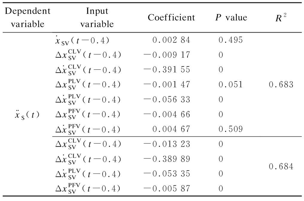
By employing the least-squares estimation method, the sensitivity parameters are calibrated with different drivers’ reaction times ranging from 0.1 to 1 s. Tab.1 summarizes the estimated optimal values of parameters and corresponding supporting statistics indicators. Notably, the linear model is statistically significant at the 99% confidence level (P<0.01). Considering that the individual driving behavior is modelled, R2 value is reasonable. Based on the supporting statistics indicators, the impact of ![]()
![]()
![]() on the SV’s longitudinal acceleration during the DLCP process is insignificant and can be ignored. This can account for these input variables having strong correlations with remaining input variables. Therefore, original model Eq.(1) is simplified into
on the SV’s longitudinal acceleration during the DLCP process is insignificant and can be ignored. This can account for these input variables having strong correlations with remaining input variables. Therefore, original model Eq.(1) is simplified into
(2)
The estimated parameters and supporting statistics indicators for the simplified model are also summarized in Tab.1.
Tab.1 Summary of original and simplified modelling
results for SV
Dependentvariable InputvariableCoefficientP valueR2¨xS(txSV(t-0.4)0.002 840.495ΔxCLVSV(t-0.4)-0.009 170xCLVSV(t-0.4)-0.391 550ΔxPLVSV(t-0.4)-0.001 470.051xPLVSV(t-0.4)-0.056 330ΔxPFVSV(t-0.4)-0.004 660xPFVSV(t-0.4)0.004 670.509ΔxCLVSV(t-0.4)-0.013 230xCLVSV(t-0.4)-0.389 890xPLVSV(t-0.4)-0.053 350ΔxPFVSV(t-0.4)-0.005 8700.6830.684
3.2 Model validation
The effectiveness of the above-proposed model in replicating real longitudinal driving behavior during DLCP period is validated using the MOE (model of effectiveness) indices: MAE (mean absolute error) and RMSE (root mean square error). Their formulations are

(3)

(4)
where M represents the number of all samples;m represents the observation instant number of sample subset; the superscript “real” and “sim” denote the values from the real dataset and the proposed model, respectively; x can be position p, velocity v and acceleration a.
Tab.2 exhibits the validation results of SV. Both model errors using the calibration and validation samples are within an acceptable range based on the table. Therefore, the proposed acceleration model can replicate the longitudinal driving behavior of SV during DLCP period with good performance. From Tab.2, it can be found that the MAE and RMSE of p, v and a have great differences. This can be explained by the fact that the variation range of positions, velocity and acceleration differ greatly during the DLCP period.
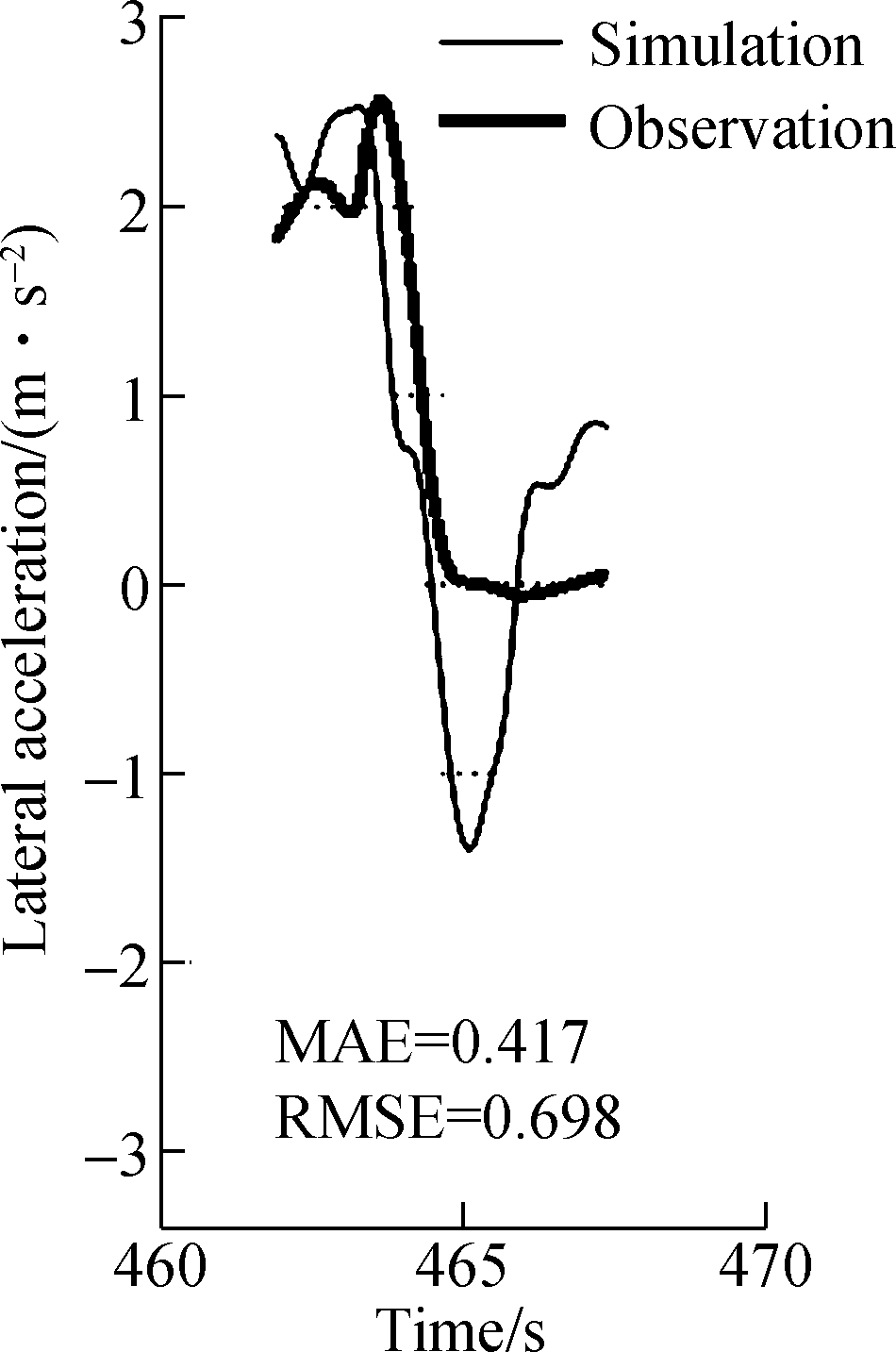
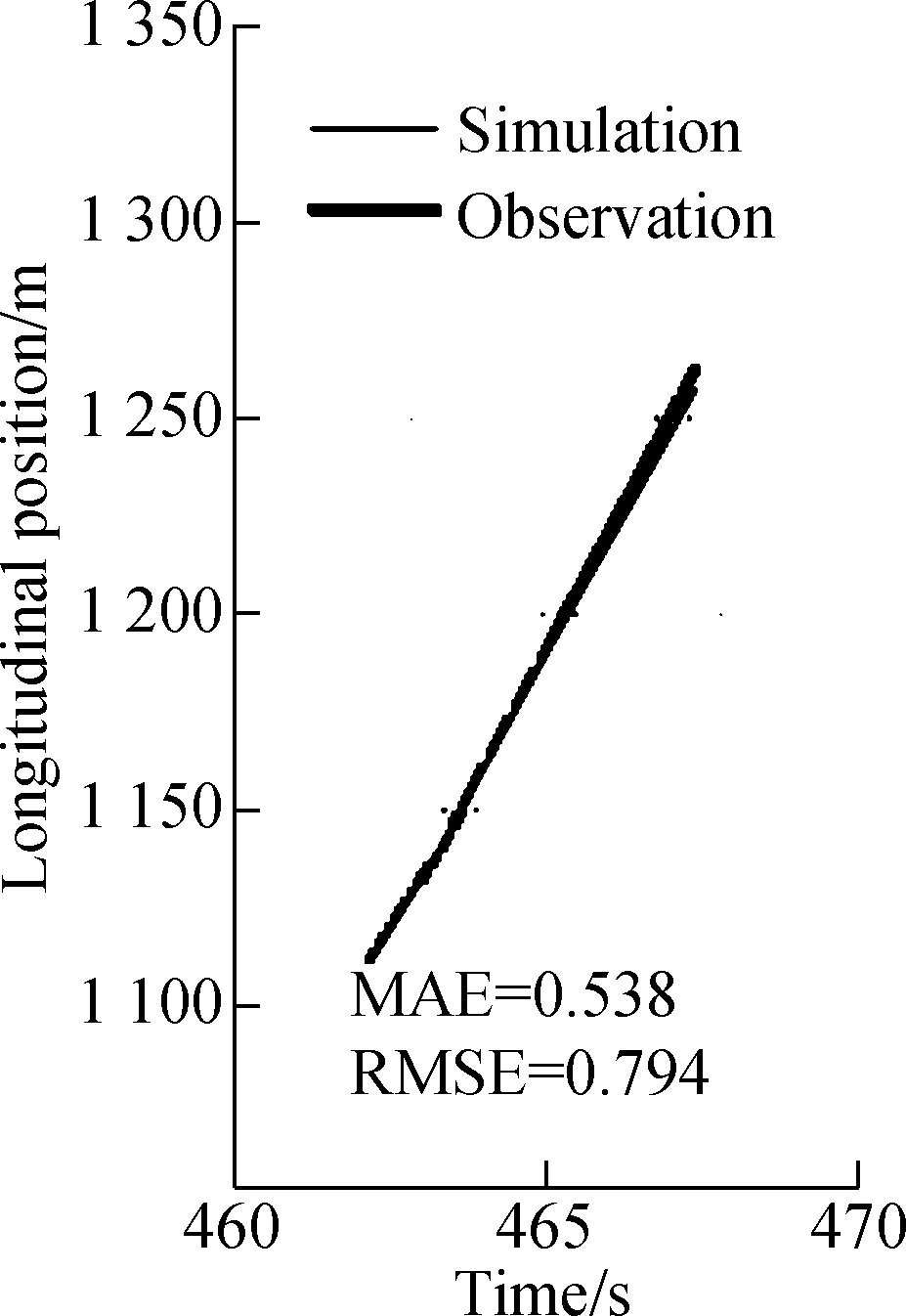
Meanwhile, we used the simplified proposed model to simulate three real DLCP trajectories selected from the aforementioned dataset. One trajectory of SV with a longitudinal speed of 7.455 m/s at the beginning of the DLCP period is selected randomly. The actual observed DLCP trajectory is used as a reference trajectory for the comparison. Fig.4 presents the simulation results of acceleration,
Tab.2 Summary of validation results for SV

ModelCalibrationp/mv/(m·s-1)a/(m·s-2)Validationp/mv/(m·s-1)a/(m·s-2)OriginalMAE4.9371.3460.8525.8341.3700.902RMSE6.5131.5991.1787.4871.6251.244SimplifiedMAE5.2181.4020.8596.1751.4360.909RMSE6.9241.6631.1787.9501.6931.244
velocity and position trajectory for the simplified proposed model. From Fig.4, errors are acceptable compared with the similar work on validations for car following models[28].
(a) 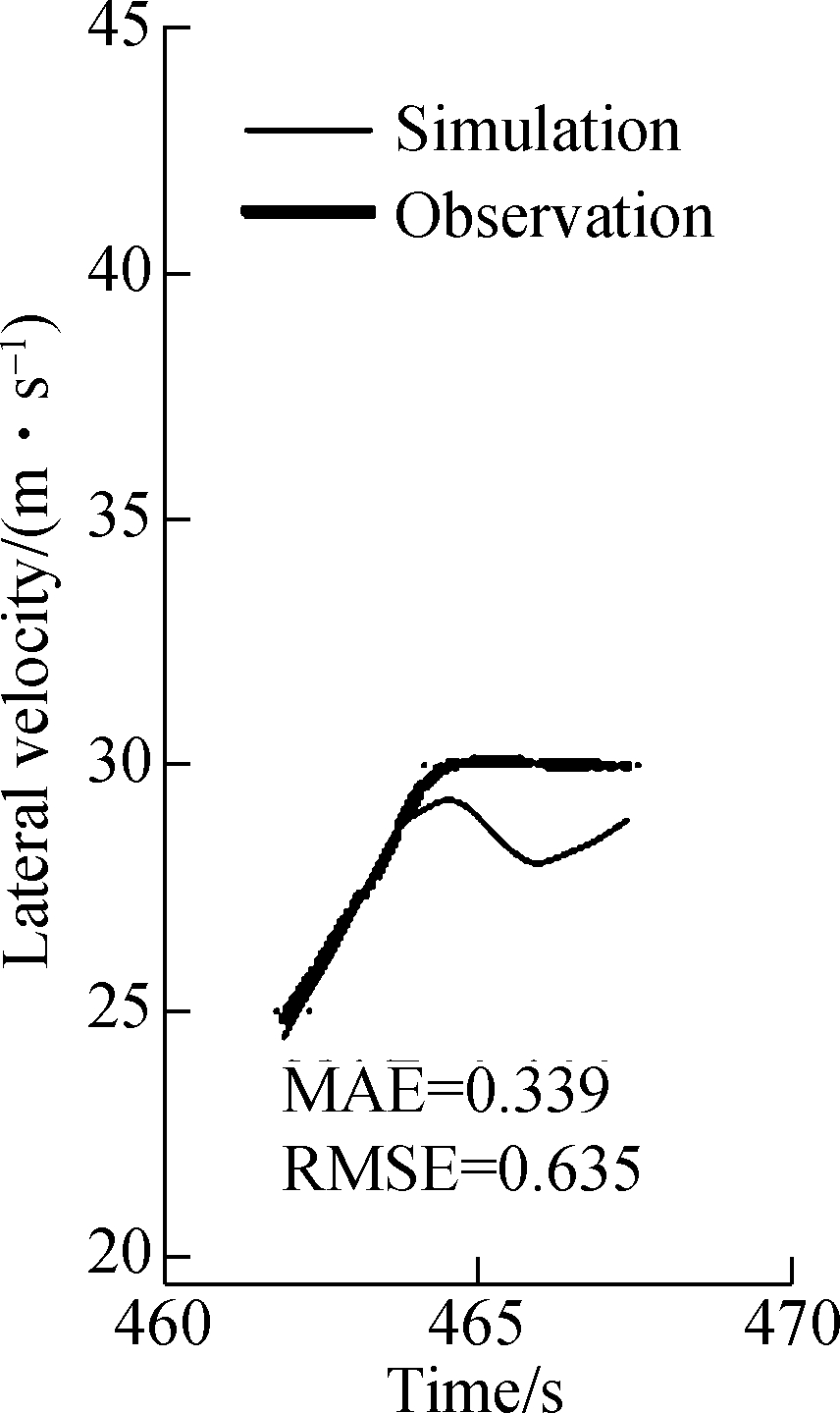
(b)
(c)
Fig.4 Simulated acceleration trajectory of SV with an initial velocity of 7.455 m/s.
(a) Acceleration trajectory;(b) Velocity trajectory; (c) Position trajectory
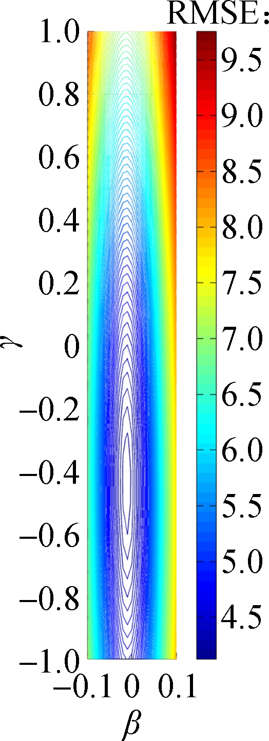
The following analysis focuses on the change of one of the MOEs, i.e. RMSE, with a subtle variation of calibrated parameters for the simplified model, since it can be seen as an indicator of the robustness of the calibration results. In Fig.5, the variations of parameters β in relation with the other three parameters γ, ω and δ for the average of all SV samples are analyzed. Here, β is restricted to the interval [-0.1, 0.1], γ to [-1 1],ω to [-0.1 0.1], δ to [-0.01 0.01]. Note the symmetry in each sub-figure, which is due to the linear effect of the model. The visual relationships between β and the other three parameters are sufficient to suggest that the calibrations for γ, ω and δ are robust, except β.
(a) 
(b) 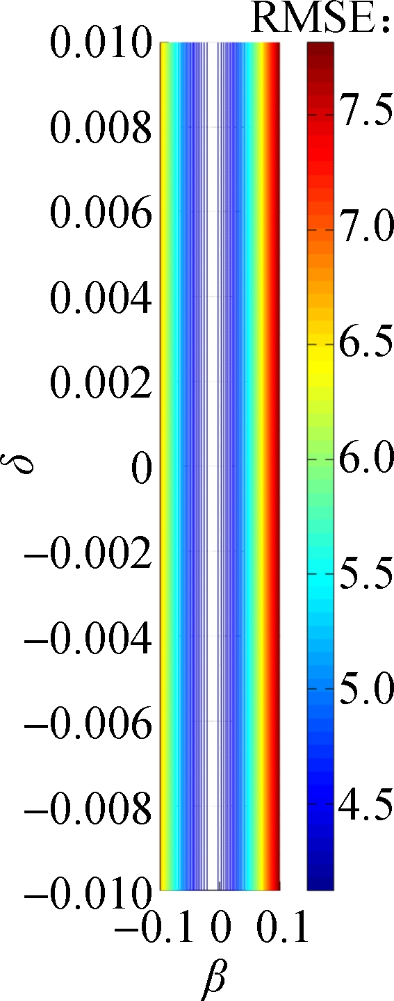 (c)
(c)
Fig.5 Sensitivity of parameters around the found minimum RMSE of the simulated acceleration for SV.
(a) Change of γ with β;(b) Change of ω with β; (c) Change of δ with β
4 Acceleration Model of following putative Vehicle during DLCP Process
In Section 3, it is mentioned that the target gap will enlarge the continuity during the DLCP period. In this section, how the target gap changes in detail will be discussed. First, the velocities of PFV versus PLV from all the observations are plotted in Fig.6. These plots reveal a obvious linear trend with a positive slope and a negative intercept. The relationship between the optimal velocity of PFV and PLV is assumed to be a linear model, which is represented by
(5)
where ![]() represents the optimal velocity of PFV during DLCP period. Based on the least-squares estimation method, p0 and p1 are estimated to be -3.708 0 and 0.933 2, respectively. Supporting statistics R2 for the linear model is 0.77, which is quite reasonable.
represents the optimal velocity of PFV during DLCP period. Based on the least-squares estimation method, p0 and p1 are estimated to be -3.708 0 and 0.933 2, respectively. Supporting statistics R2 for the linear model is 0.77, which is quite reasonable.
Considering the slope of fitted straight line p1 is close to 1 (see Fig.6), the slope value presumably should be 1, and Eq.(5) is simplified into
(6)
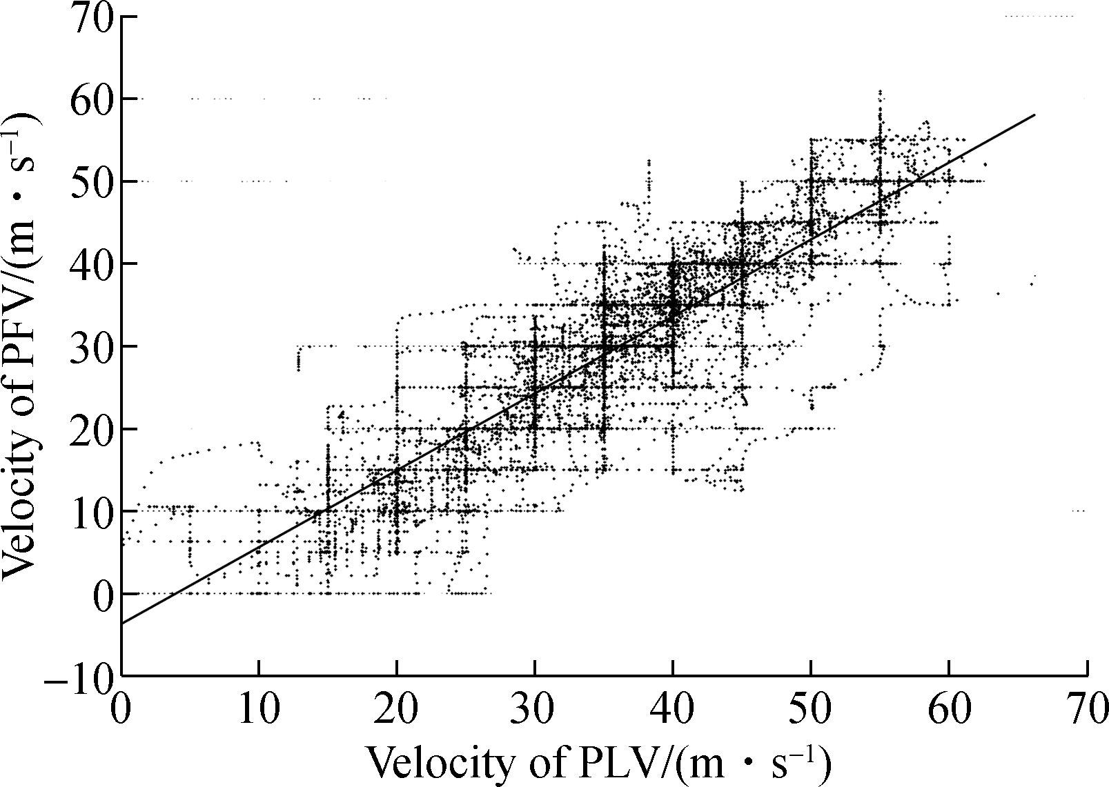
Fig.6 Velocity of PFV versus PLV
It implies that the optimal velocity of PFV relative to PLV remains stable and is equal to p0 during the DLCP period. Then, the next work is to estimate constant term p0 more accurately again. From Eq.(6), the value of p0 is equivalent to the relative velocity with PLV of PFV. The frequency histogram for the distribution of the optimal velocity of PFV relative to PLV from all observation samples is shown in Fig.7, which is consistent with the normal distribution curve obviously. Thus, the assumption that the velocity of PFV relative to PLV obeys the normal distribution is made, and the estimation of p0 with the expectation of the fitted normal distribution, i.e. N(-6.006,37.283) is also made based on the selected samples. Therefore, Eq.(6) can be rewritten as
(7)
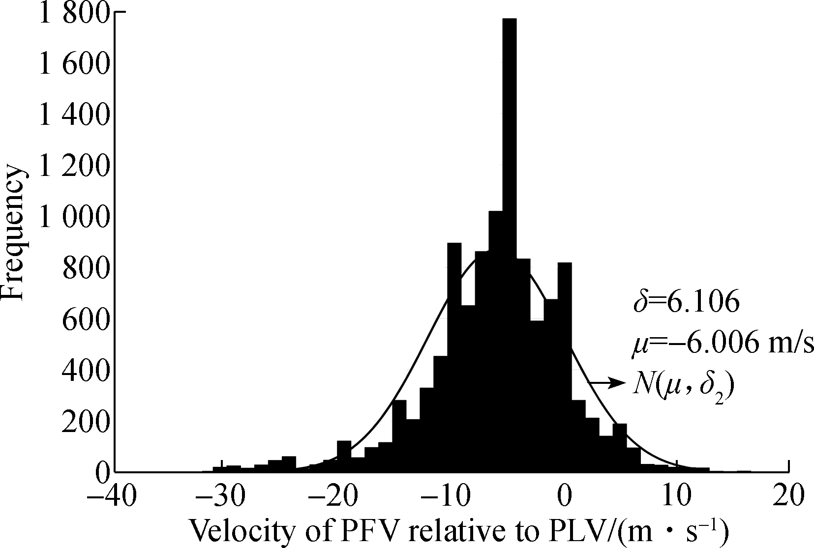
Fig.7 Distribution of velocity of PFV relative to PLV
According to Eq.(7), it can be validated that the optimal velocity of PFV is to guarantee that the target gap will be increased continuously with a stable velocity during the DLCP period.
Moreover,referring to the optimal velocity model[29] and the above-mentioned study results for lane-changing vehicle,an acceleration model is constructed to simulate the longitudinal driving behavior of PFV during the DLCP process, as follows:
(8)
By substituting ![]() with Eq.(7), Eq.(8) can be simplified into
with Eq.(7), Eq.(8) can be simplified into
(9)
By using the similar calibration method with SV’s acceleration model, the values of parameters α, β, γ and T are estimated to be -0.144 14, -0.012 50, -0.101 41, and 0.4, respectively.
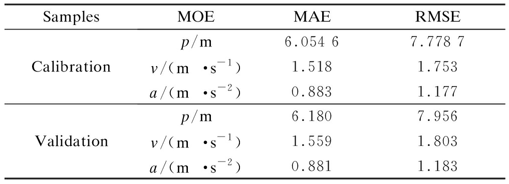
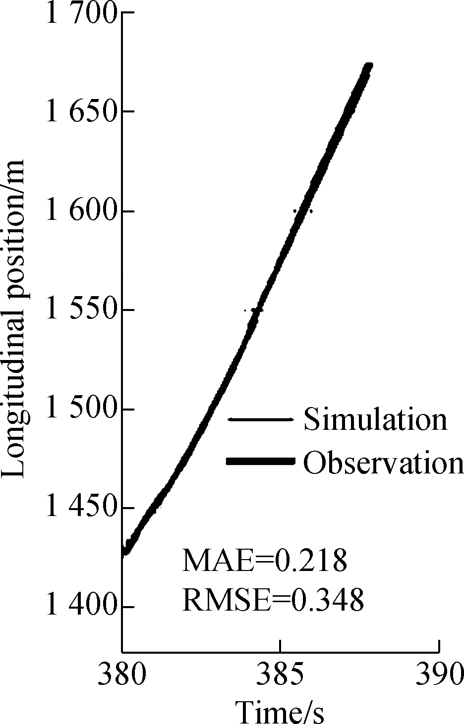
Tab.3 exhibits the validation results of PFV, which suggests that the proposed model has good performance in simulating the longitudinal driving behavior of PFV during the DLCP period. In Fig.8, likewise, the proposed model is used for PFV to simulate one real DLCP trajectory, with
Tab.3 Summary of validation results of PFV
SamplesMOEMAERMSECalibrationp/m6.054 67.778 7v/(m·s-1)1.5181.753a/(m·s-2)0.8831.177Validation p/m6.1807.956v/(m·s-1)1.5591.803a/(m·s-2)0.8811.183

(a) 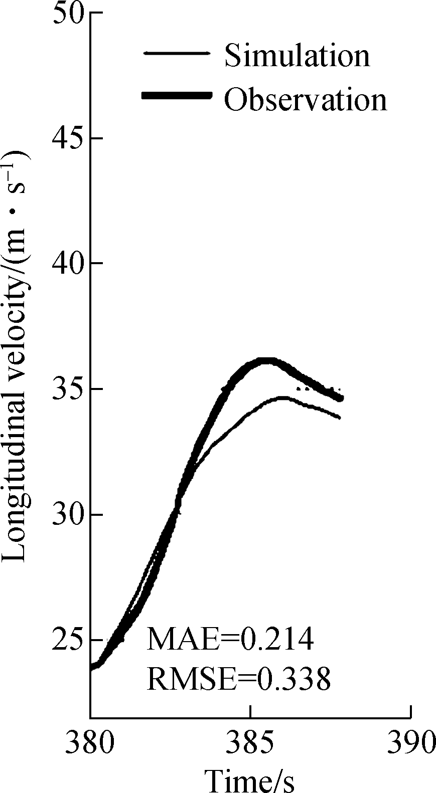
(b)
(c)
Fig.8 Simulated trajectory of PFV with an initial velocity of 7.146 m/s.
(a) Acceleration trajectory;(b) Velocity trajectory; (c) Position trajectory
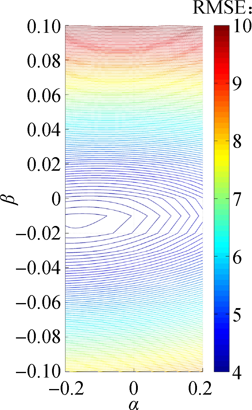
an initial longitudinal speed of 7.146 m/s. The simulation results are acceptable as well. In Fig.9, the variation of parameters α in relation with the other two parameters β and γ for the average of all PFV samples are analyzed. α is restricted to the interval [-0.2, 0.2], β to [-0.1, 0.1],γ to [-1, 1]. Here, α seems to be robust in the restricted interval, while β and γ appear to be robust only in the smaller intervals [-0.04, 0.02] and [-0.4, 0.2], respectively.
5 Conclusions
1) Two acceleration models are proposed to simulate the car-following behavior of SV and PFV during the DLCP period. Besides, two simple but practical methods are employed to identify both the starting and ending point of DLCP process, respectively. The validation results of the
(a) 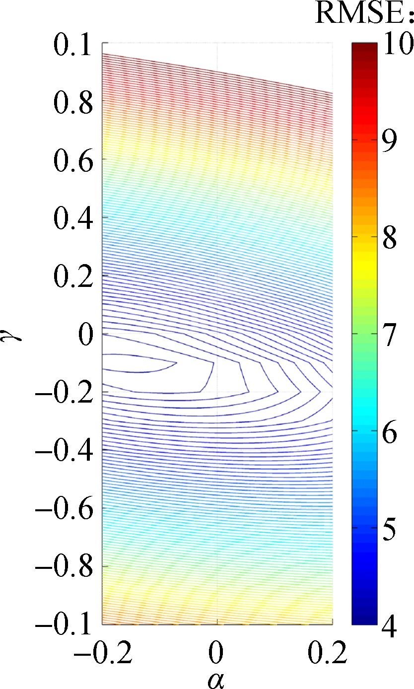
(b)
Fig.9 Sensitivity of parameters around the found minimum RMSE of the simulated acceleration for PFV.
(a) Change of β with α;(b) Change of γ with α
linear acceleration models for SV are very close and quite acceptable compared with similar calibrations of car-following models. Moreover, the parameter sensitivity analysis suggests that the calibrated model is robust with subtle input variable observation errors.
2) The PFV acceleration model by referring to the optimal velocity model is proven to have good performance in simulating car-following behavior during the DLCP period as well. The calibrated optimal velocity function for PFV acceleration model suggests that PFV is expected to increase the target gap continuously with a stable optimal velocity relative to PLV.
3) In traditional microscopic simulation models, the DLCP process is considered to be the same as the car following phase and the longitudinal motion of lane-changing vehicle during DLCP process is simulated with regular car-following models. On the basis of identification of the starting and ending point of DLCP process from real trajectory data, the construction of the decision-making model for starting and ending the DLCP process will be our next work. The data source used in this study is limited to one dataset in NGSIM data. More datasets will be calibrated in order to validate our models in the future.
[1] Zheng Z D. Recent developments and research needs in modeling lane changing[J]. Transportation Research Part B: Methodological, 2014, 60: 16-32. DOI:10.1016/j.trb.2013.11.009.
[2] Rahman M, Chowdhury M, Xie Y, et al. Review of microscopic lane-changing models and future research opportunities[J]. IEEE Transactions on Intelligent Transportation Systems, 2013, 14(4): 1942-1956. DOI:10.1109/tits.2013.2272074.
[3] Gipps P G. A model for the structure of lane-changing decisions[J]. Transportation Research Part B: Methodological, 1986, 20(5): 403-414. DOI:10.1016/0191-2615(86)90012-3.
[4] Halati A, Lieu H, Walker S. CORSIM-corridor traffic simulation model [C]//Transportation Research Board Annual Meeting. Washington, DC, USA,1997: 570-576.
[5] Hidas P. SITRAS: A simulation model for ITS applications [C]//Towards the New Horizon Together Word Congress on Intelligent Transport Systems. Seoul, Korea, 1998: 3170-3176.
[6] Rickert M, Nagel K, Schreckenberg M, et al. Two lane traffic simulations using cellular automata[J]. Physica A: Statistical Mechanics and its Applications, 1996, 231(4): 534-550. DOI:10.1016/0378-4371(95)00442-4.
[7] Liu H, Xin W, Adams Z, et al. A game theoretical approach for modeling merging and yielding behaviour at freeway on-ramp sections[M]. London: Elsevier, 2007:197-211.
[8] Ahmed K I. Modeling drivers’ acceleration and lane changing behavior[D]. Cambridge, USA: Massachusetts Institute of Technology, 1999.
[9] Toledo T, Koutsopoulos H N, Ben-Akiva M. Integrated driving behavior modeling[J]. Transportation Research Part C: Emerging Technologies, 2007, 15(2): 96-112. DOI:10.1016/j.trc.2007.02.002.
[10] Hunt J G, Lyons G D. Modelling dual carriageway lane changing using neural networks[J]. Transportation Research Part C: Emerging Technologies, 1994, 2(4): 231-245. DOI:10.1016/0968-090x(94)90012-4.
[11] Yan F, Eilers M, Baumann M, et al. Development of a lane change assistance system adapting to driver’s uncertainty during decision-making[C]// Proceedings of the 8th International Conference on Automotive User Interfaces and Interactive Vehicular Applications. ACM, 2016:93-98. DOI:10.1145/3004323.3004334.
[12] Das S. A fuzzy logic model of freeway driver behavior [C]// International ICSC Congress on Computational Intelligence Methods and Applications. Rochester, NY, 1999: 5-11.
[13] Kesting A, Treiber M, Helbing D. General lane-changing model MOBIL for car-following models[J].Transportation Research Record: Journal of the Transportation Research Board, 2007, 1999: 86-94.DOI:10.3141/1999-10.
[14] Moridpour S, Sarvi M, Rose G. Modeling the lane-changing execution of multiclass vehicles under heavy traffic conditions[J]. Transportation Research Record: Journal of the Transportation Research Board, 2010, 2161:11-19. DOI:10.3141/2161-02.
[15] Papadimitriou I, Tomizuka M. Fast lane changing computations using polynomials[J]. Proceedings of the 2003 American Control Conference.Denver, USA, 2003:48-53. DOI:10.1109/acc.2003.1238912.
[16] Kou C, Machemehl R B. Modeling driver behavior during merge maneuvers[D]. Austin, Texas, USA: Southwest Region University Transportation Center, University of Texas, 1997.
[17] Wan X, Jin P, Yang F, et al. Modeling vehicle interactions during merge in congested weaving section of freeway ramp[J]. Transportation Research Record: Journal of the Transportation Research Board, 2014, 2421: 82-92. DOI:10.3141/2421-10.
[18] Wang H, Li Y, Wang W. Modeling lane changing execution on the basis of car following theory[C]//Transportation Research Board Annual Meeting. Washington, DC, USA, 2015: 2651-2662.
[19] Hidas P. Modelling vehicle interactions in microscopic simulation of merging and weaving[J]. Transportation Research Part C: Emerging Technologies, 2005, 13(1): 37-62. DOI:10.1016/j.trc.2004.12.003.
[20] Sun D J, Kondyli A. Modeling vehicle interactions during lane-changing behavior on arterial streets[J].Computer-Aided Civil and Infrastructure Engineering, 2010, 25(8): 557-571. DOI:10.1111/j.1467-8667.2010.00679.x.
[21] Schakel W, Knoop V, van Arem B. Integrated lane change model with relaxation and synchronization[J].Transportation Research Record: Journal of the Transportation Research Board, 2012, 2316: 47-57.DOI:10.3141/2316-06.
[22] Wan X, Jin P, Zheng L, et al. Speed synchronization process of merging vehicles from the entrance ramp[J].Transportation Research Record: Journal of the Transportation Research Board, 2013, 2391: 11-21.DOI:10.3141/2391-02.
[23] Park H, Oh C, Moon J,et al. Development of a lane change risk index using vehicle trajectory data[J].Accident Analysis & Prevention, 2018, 110: 1-8.
[24] Cleveland W S. LOWESS: A program for smoothing scatterplots by robust locally weighted regression[J].The American Statistician, 1981, 35(1): 54. DOI:10.2307/2683591.
[25] Zheng Z, Ahn S, Chen D, et al. The effects of lane-changing on the immediate follower: Anticipation, relaxation, and change in driver characteristics[J]. Transportation Research Part C: Emerging Technologies, 2013, 26: 367-379. DOI:10.1016/j.trc.2012.10.007.
[26] Ghaffari A, Khodayari A, Hosseinkhani N, et al. The effect of a lane change on a car-following manoeuvre: Anticipation and relaxation behaviour [J]. Proceedings of the Institution of Mechanical Engineers, Part D: Journal of Automobile Engineering, 2015,229(7): 809-818.
[27] Sun D J. Alane-changing model for urban arterial streets[D]. Gainesville, FL, USA:University of Florida,2009.
[28] Ossen S J L. Longitudinal driving behavior: Theory and empirics[D]. Cambridge, USA: Delft University of Technology, 2008.
[29] Bando M, Hasebe K, Nakayama A, et al. Dynamical model of traffic congestion and numerical simulation[J]. Physical Review E, 1995, 51(2): 1035-1042.DOI:10.1103/physreve.51.1035.