Bearings are the most common mechanical parts in rotating machinery. According to statistics, 30% of rotating machinery failures and 40% of motor failures are related to rolling bearings[1-3]. Obviously, bearings are one of the most fault-prone parts in mechanical equipment, so the fault diagnosis of the rolling bearings is necessary.
Traditional fault diagnosis methods are usually divided into three steps: 1) Fault signal acquisition; 2) Feature extraction; 3) Fault diagnosis. There are many research results based on traditional fault diagnosis methods. Abbasion et al.[4] firstly used wavelet analysis to preprocess the vibration signal of the motor bearing, which reduced the noise in the signal, and then they used the support vector machine to classify the faults. Han et al.[5] used LMD to decompose the original signal, then extracted the energy entropy and sample entropy of each product function, and finally used the support vector machine for fault diagnosis. Wu[6] applied wavelet packet decomposition to analyze multi-resolution bearing signals, and compared three diagnosis methods which are the BP, RBF and Elman network. However, manually extracting features requires prior knowledge to achieve better diagnostic results.
Convolution neural network (CNN) is one of the methods of deep learning. It has powerful information mining capability and can automatically extract features, and some achievements have been obtained by using CNN in the field of fault diagnosis. You et al.[7] used CNN to extract the features of vibration signals from rolling bearing, then input the extracted features into SVM for fault identification. Ding et al. [8] performed wavelet packet transform on the vibration signal to obtain its grayscale images, and then used them as the input of CNN to identify faults. Chen et al.[9] used 2DCNN to diagnose faults in the gearbox, whose input matrix is 16×16, reconstructed by 256 statistical features including RMS, standard deviation, skewness, kurtosis, rotation frequency and load. However, the method did not utilize the information mining capability of CNN. Guo et al.[10] proposed an adaptive CNN model, which can speed up the convergence rate to a certain extent and improve the recognition rate by changing the learning rate automatically. Janssens et al. [11] utilized 2DCNN to identify the patterns of four types of rotating machinery faults whose input was derived from DFT (discrete Fourier transform) of vibration acceleration signals acquired by two acceleration sensors. Wang et al.[12] applied the PSO algorithm to optimize the hyper-parameters of the CNN model, so that the network can adaptively learn more rules of the data set. Although some of the methods mentioned above have more or less achieved some good results, they still have the following deficiencies: 1) The traditional fault diagnosis method needs to use prior knowledge to extract features and how to exploit the ability of CNN to extract signal features automatically is worth studying; 2) The two-dimensional convolution kernel of a classical 2DCNN will disrupt the periodicity of fault signal, which renders the extracted features inconspicuous, resulting in inaccurate final diagnostic results; 3) There are many hyper-parameters in the CNN, and the selection of hyper-parameters affects the final effect of the algorithm. Therefore, it is necessary to optimize the hyper-parameters.
In this paper, combining the genetic algorithm and convolution neural network with one-dimensional large convolution kernel can solve the above problems, and we call the hybrid algorithm GA-1DLCNN. A comparative experiment is carried out to prove the effectiveness of the method. In addition, another experiment verifies that large convolution kernels have advantages over small convolution kernels and two-dimensional convolution kernels.
1 Basic Theory
1.1 Theory of CNN
The convolution layer and pool layer of CNN make it superior to traditional neural networks. Different convolution layers contain different numbers of convolution kernels. The convolution kernels continuously move on the feature maps passed on from the previous layer. During the movement, the convolution kernel is continuously convoluted with the overlapping data, and the output of the convolution layer is finally obtained. This constantly moving operation of the single convolution kernel also causes CNN to have the characteristic of weight sharing. Compared with the disadvantage of excessive weights in fully-connected networks, the sharing of the weights of CNN can reduce network parameters, which reduces computational complexity and avoids network overload caused by excessive weights. The following part describes the forward propagation algorithm of CNN.
Here, suppose that the input of the convolution layer is x∈RA×B, where A is the number of samples, B is the data dimension, and the output of the convolution layer is calculated as
(1)
where Ol-1 denotes the output of the first feature map of the first layer; ![]() represents the j-th feature map of the l-th layer; *denotes a convolution calculation; f denotes an activation function, which mainly includes modified linear unit (Relu) and sigmoid function; bl is the offset item.
represents the j-th feature map of the l-th layer; *denotes a convolution calculation; f denotes an activation function, which mainly includes modified linear unit (Relu) and sigmoid function; bl is the offset item.
In general,the pooling operation on the feature data is a nonlinear sampling method after the convolution operation. Through the pooling operation, the matrix size of the feature map can be effectively reduced, thereby reducing the parameters in the last fully connected layer. Its formula is
xl=down(xl-1)
(2)
where xl-1 denotes the output of the previous convolution layer; down( ) denotes the sampling operation, and the most commonly used sampling operation is the max-pooling, that is, taking the maximum value of the local area.
The CNN consists of pairs of convolution and pooling layers. Normally, the fully connected layer follows the last pooling layer. The fully connected layer of CNN is the same as that of traditional artificial neural networks. The number of full connection layers can be determined according to the specific conditions. The last layer of CNN is the softmax layer. The softmax layer is the classification layer of CNN. The number of neurons on this layer is equal to that of the categories that need to be classified. The formula on the softmax layer is


(3)
where O represents the result of the output layer, which is the output category; C is the number of failure categories.
Fig.1 shows the 1DLCNN model, and it can directly input the original one-dimensional vibration signal into the model. The model has two convolution layers and two pooling layers. From pooling layer 2 to the fully connected layer, each map of the pooling layer needs to be connected, and the output layer finally classifies the fault categories.
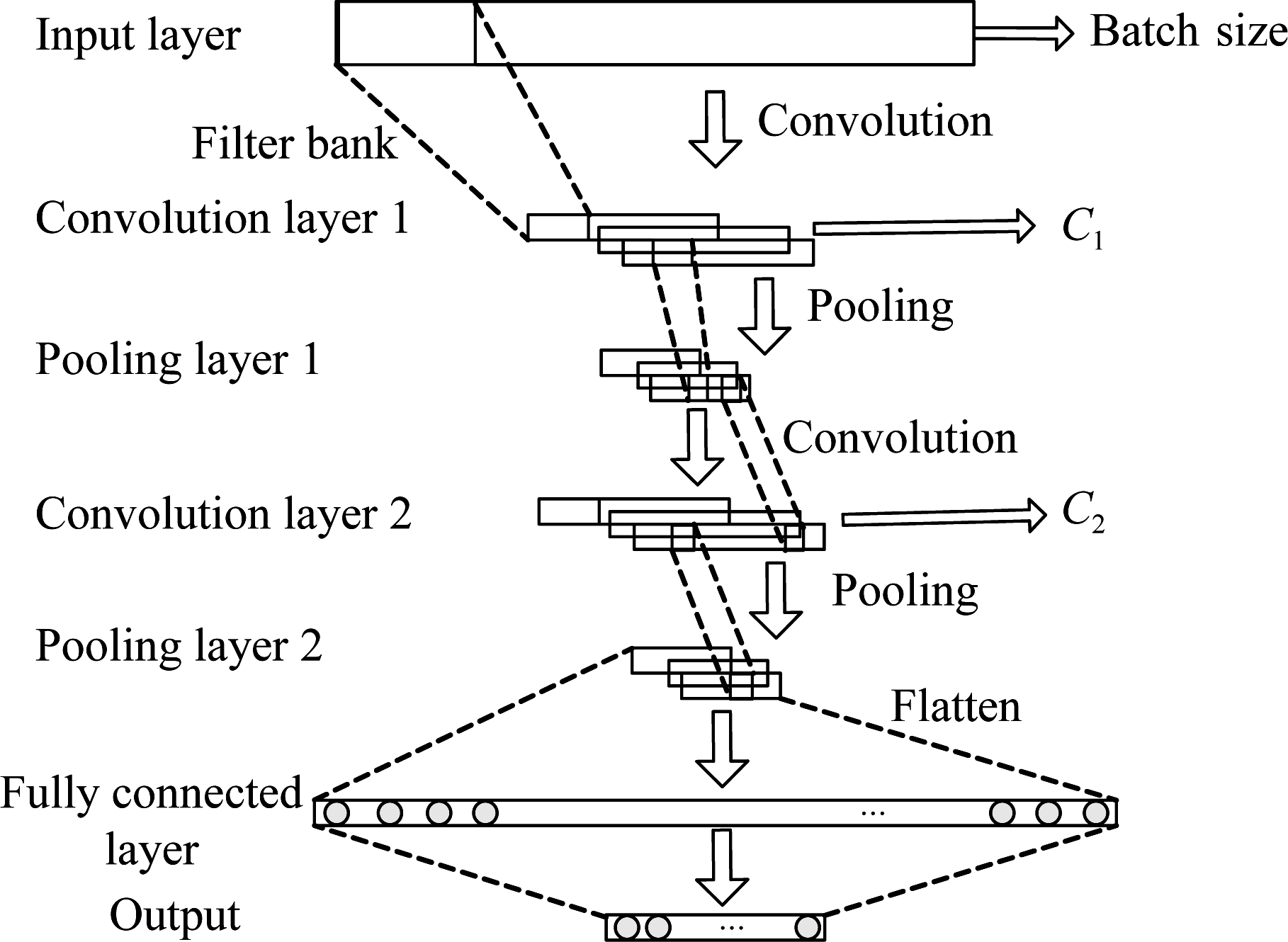
Fig.1 1DLCNN model construction
1.2 Hyper-parameter optimization by genetic algorithm
The CNN model has many hyper-parameters, and different hyper-parameter combinations can lead to varying model generalization performances. As there are many hyper-parameters in the model, different hyper-parameter combinations will vary each model performance. In order to obtain the optimal hyper-parameter combination, this paper proposes a new method combining the genetic algorithm with 1DLCNN,which is called the GA-1DLCNN method. On the one hand, the algorithm can play the role of 1DLCNN without manually extracting features (input raw data directly). On the other hand, it can exert the optimization characteristics of the genetic algorithm. The parameters needed to be optimized are the kernel number of the first convolution layer C1, the kernel number of the second convolution layer C2, the learning rate ε, the batch size B, and the number of iterations I.
The genetic algorithm is a method of searching for optimal solutions by simulating natural evolutionary processes, which uses the fitness function and probability transformation rules to guide the search direction. The basic operations of the genetic algorithm include selection, crossover, and mutation. The specific optimization processes are as follows:
1) Initializing the population and encoding. A group Xm×n is randomly generated, and each individual X1×n represents a hyper-parameter distribution. Here, n represents the number of hyper-parameters, and m is the initial population size. The encoding is shown in Fig.2.
Fig.2 Chromosome coding
2) Determining the fitness function. The squared reconstruction error of the training sample of 1DLCNN model is used as the fitness function, and its formula is as
(4)
where o=(o1,o2,…,oC) is the actual output(obtained by Eq.(3)); the expected output is y=(y1,y2,…,yC). In this paper, one hot encoding is used to indicate expected output, for example, (0,0,0,1) means this is the fourth category.
3) Selecting. The roulette method based on the fitness ratio selection strategy is used. The probability of selection pq for each individual q is
(5)

(6)
where Fq is the fitness value of the individual; λ is the coefficient.
4) Cross operation. Since the individual uses real number coding, the cross operation uses the real number crossing method, and the cross operation method of the u-th chromosome au and the v-th chromosome av in the w-th place is
(7)
where b is a random number between [0, 1].
5) Variation. New individuals are generated based on the probability of mutation.
6) Calculate the fitness value and determine whether the maximum evolution algebra is reached, otherwise return to step 3).
After the optimization of the genetic algorithm is completed, the obtained optimal individual is utilized as the hyper-parameter combination of 1DCNN.
2 Rotating Machinery Fault Diagnosis Method Based on GA-1DLCNN
The flow chart of the fault diagnosis method based on GA-1DLCNN is shown in Fig.3. The specific steps are as follows:
1) Collect the fault signal, then intercept signals at equal length to obtain multiple sets of samples, and randomly separate the training set and the test set.
2) Generate an initial population. Set the number of populations and the max generation.
3) Train each 1DLCNN model, and the fitness function is obtained by Eq.(4).
4) Sequentially select, cross, and mutate operations to generate new populations, determine whether the max generation is reached. If the discriminant condition is met, output the optimal network hyper-parameter, otherwise, repeat steps 3) and 4) until the discriminant condition is satisfied.
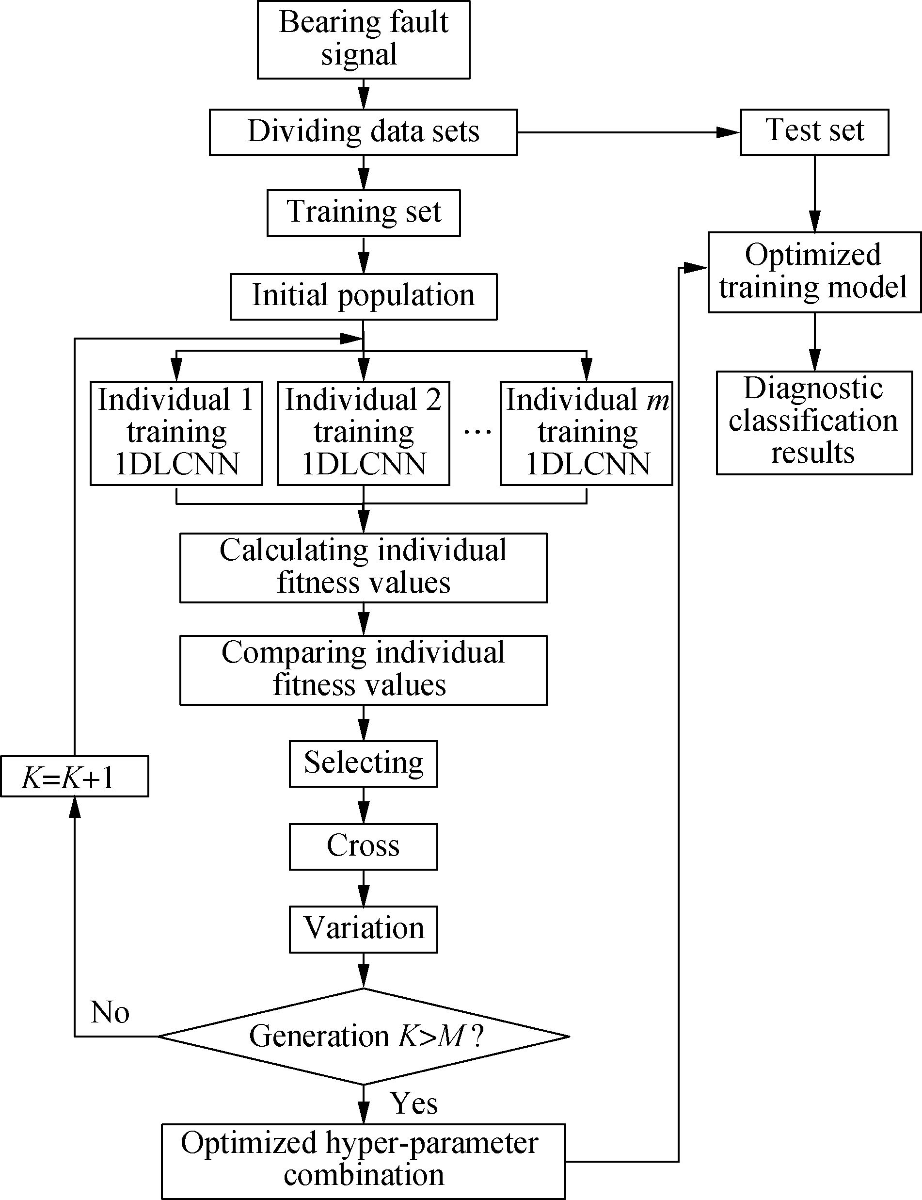
Fig.3 Fault diagnosis process of rotating machinery based on GA-1DLCNN
5) Input the test set into the optimized model to obtain the fault classification results.
3 Experimental Verification and Discussion
3.1 Experimental data description
The experimental data comes from the bearing failure experiment of Case Western Reserve University. The sampling frequency is 12 kHz and the failures are divided into 3 types: Inner race failure, outer race failure and ball failure. Each failure type has three fault sizes of 0.007, 0.014, and 0.021 mm, respectively, and a total of 9 fault categories were obtained, namely, label1, label2, ... , label9. In this experiment, the data length of each sample was set to be 1 024, and 200 samples can be obtained for each fault. A total of 1 800 samples can be obtained, and 1 200 samples were randomly selected as training samples, and another 600 samples were used as test samples (test samples did not participate in training).
3.2 Test results and analysis
3.2.1 Analysis of the proposed method
The simulation for 1DLCNN is performed in Tensorflow, a Google open deep learning platform. In addition,the NVIDIA GTX1050Ti GPU is used to accelerate algorithm training. In the evolution process of the genetic algorithm, the number of populations is set to be 5, the max generation is 10, the selection probability is 0.1, the crossover probability is 1, and the probability of mutation is 0.2[13].The results of hyper-parameters optimized by the genetic algorithm are shown in Tab.1. The results of each generation of the genetic algorithm are shown in Fig.4. As the generation continues to increase, the results become increasingly accurate and the recognition rate of the final model reaches 99.83%. Fig.5 shows a confusion matrix of misclassfication. The X-axis is the target category, and the Y-axis is the calculated category. When the target category is the same as the calculated category, the value at the intersection is increased by 1. So, according to Fig.5, the misclassification of each category can be obtained. Only one of 68 samples of category 1 is misclassified into category 1, and the other eight categories are all classified correctly.
Tab.1 Optimal hyper-parameters by genetic algorithm
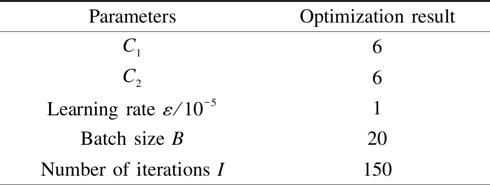
ParametersOptimization resultC16C26Learning rate ε/10-51Batch size B20Number of iterations I150
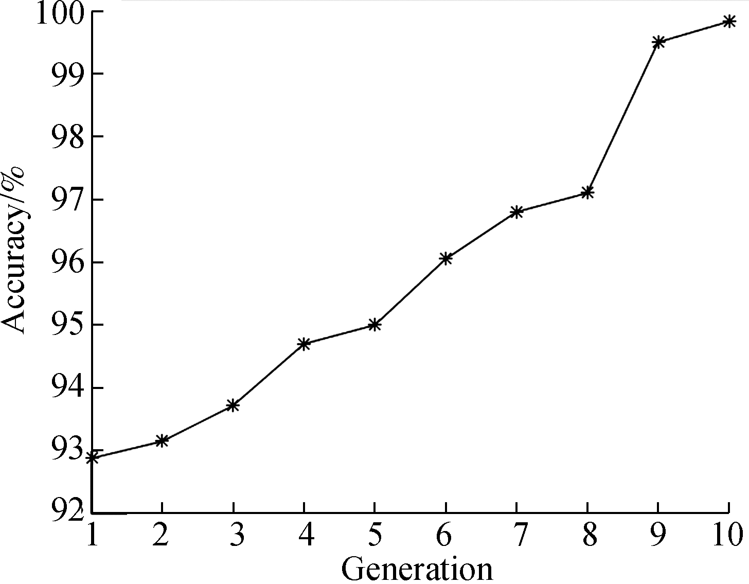
Fig.4 Genetic algorithm optimization process

Fig.5 Confusion matrix of misclassification
3.2.2 Comparison with traditional methods
Feature extraction and the classifiers are two key points of traditional fault diagnosis methods, which affect the final result greatly. In this comparison experiment,the feature extraction methods used are: 1) Time-frequency mixed statistical indicators (TMSI); 2) Wavelet packet decomposition(WPD); 3) Empirical mode decomposition(EMD). The classifiers used contain BP, SVM and stacked auto-encoder (SAE). 10 time domain statistical indicators and 5 frequency domain statistical indicators are selected as time-frequency mixed statistical features[14]. The wavelet packet decomposition decomposed each fault signal into three layers, and a total of eight different frequency band signals were obtained. The energy value of each frequency band was taken as its feature[15], and therefore, 8 features were acquired in total. The EMD decomposed the sample signal into six IMF components[16], and extracted the time-frequency mixed statistical indicators[14] as features for each component. The comparison results are shown in Tab.2. The method proposed in this paper is more advantageous than the traditional methods of extracting features and identification.
3.2.3 Further comparison with classical CNN
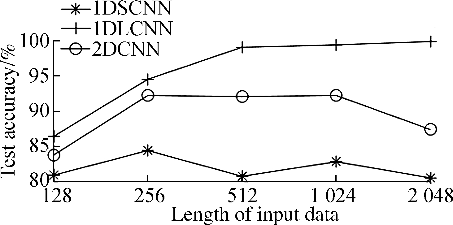
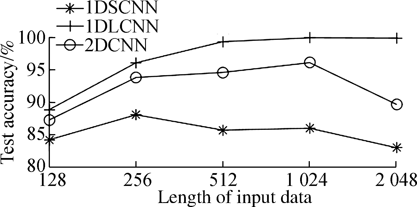
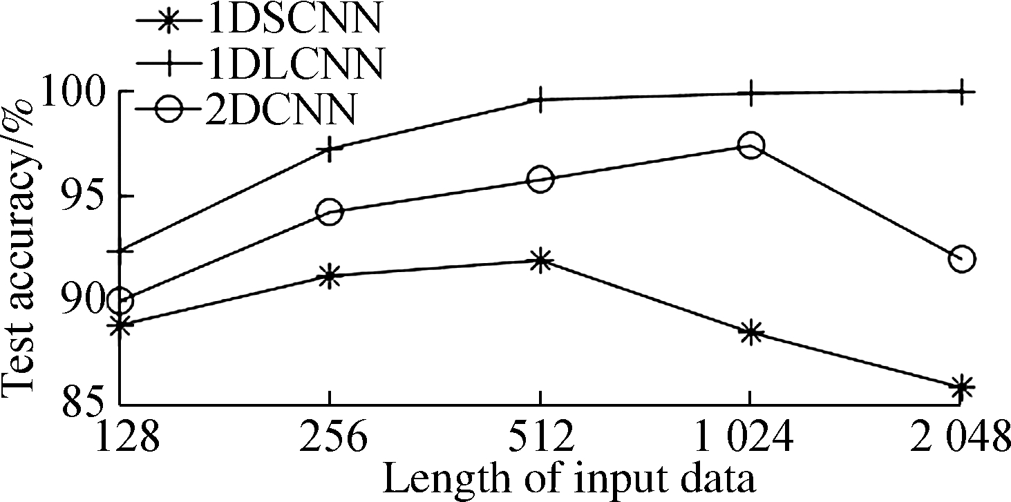
In order to more comprehensively verify the effectiveness of a one-dimensional large-size convolution kernel, a large number of experimental comparisons have been set out, in which the parameters that need to be changed include the length of the input data and the number of iterations. In this comparison, a two-dimensional convolutional neural network(2DCNN), one-dimensional small-kernel convolution neural network (1DSCNN)are selected as the comparison algorithms. The input data length is set to be 128, 256, 512, 1 024, 2 048, respectively, and the number of iterations is set to be 50, 100, 200, 300, respectively. The number of training sets accounts for 2/3 of the total number of samples, and the number of test sets accounts for 1/3 of the total number of samples. The specific data set is divided as shown in Tab.3, and the convolution kernel parameter setting for each method is shown in Tab.4. In order to reduce the error of a single test, the average of five test results is calculated as the final result.
Tab.2 Diagnostic accuracy of different methods

MethodAccuracy/%SVM+TMSI86.5SVM+WPD87.1SVM+EMD88.9BP+TMSI94.8BP+WPD92.2BP+EMD89.8SAE+TMSI84.0SAE+WPD78.7SAE+EMD84.9Proposed method99.9
Tab.3 Data set dividing

Length ofinput dataNumber ofsamplesNumber of training samplesNumber of test samples12814 4009 6004 8002567 2004 8002 4005123 6002 4001 2001 0241 8001 2006002 048900600300
Tab.4 Corresponding convolution kernel parameter settings

Length of input dataKernel size2DCNN1DSCNN1DLCNN1283×3,5×53×1,4×121×1,21×12563×3,5×53×1,4×121×1,21×15123×3,5×53×1,4×1101×1, 101×12 0143×3,5×53×1,4×1101×1, 101×12 0483×3,5×53×1,4×1501×1, 501×1
According to Fig.6, the above experiments can verify that 1DLCNN is superior to the classic 2DCNN and 1DSCNN. The reasons are as follows: 1) In the field of image processing, the traditional two-dimensional convolution neural network directly inputs two-dimensional data into the network, and the convolution kernel used is also two-dimensional, but in the field of fault diagnosis, the fault signal is usually one-dimensional. If a one-dimensional signal is reconstructed into two-dimensional data, the two-dimensional convolution kernel is used to extract the signal characteristics, which will disturb the periodicity of the signal to some extent, so that the extracted features are not obvious, resulting in lower accuracy. 2) The larger-scale convolution kernels have a larger field of perception and the extracted features are better. Therefore, the final effect is better than that of the small convolution kernel.
(a)
(b)

(c)
(d)
Fig.6 Comparison of methods for different training times. (a) 50 training steps; (b) 100 training steps; (c) 200 training steps; (d) 300 training steps
The above comparison test also explains the effect of the input data length on the recognition rate. The above input data lengths are 128, 256, 512, 1 024, and 2 048, respectively. The general trend in Fig.6 is that as the input data length increases, the recognition rate of the model increases. Due to the fault signal having a certain periodicity, if the intercepted data length is too short relative to the period, the distribution of sample data divided into the same category will be different, reducing the classification accuracy eventually. Similarly, a too long intercepted data length will result in fewer samples, which also reduces the recognition rate. Therefore, in the field of fault diagnosis, the authors believe that when the data volume is sufficient, the input data length can be increased as much as possible, which can improve recognition.
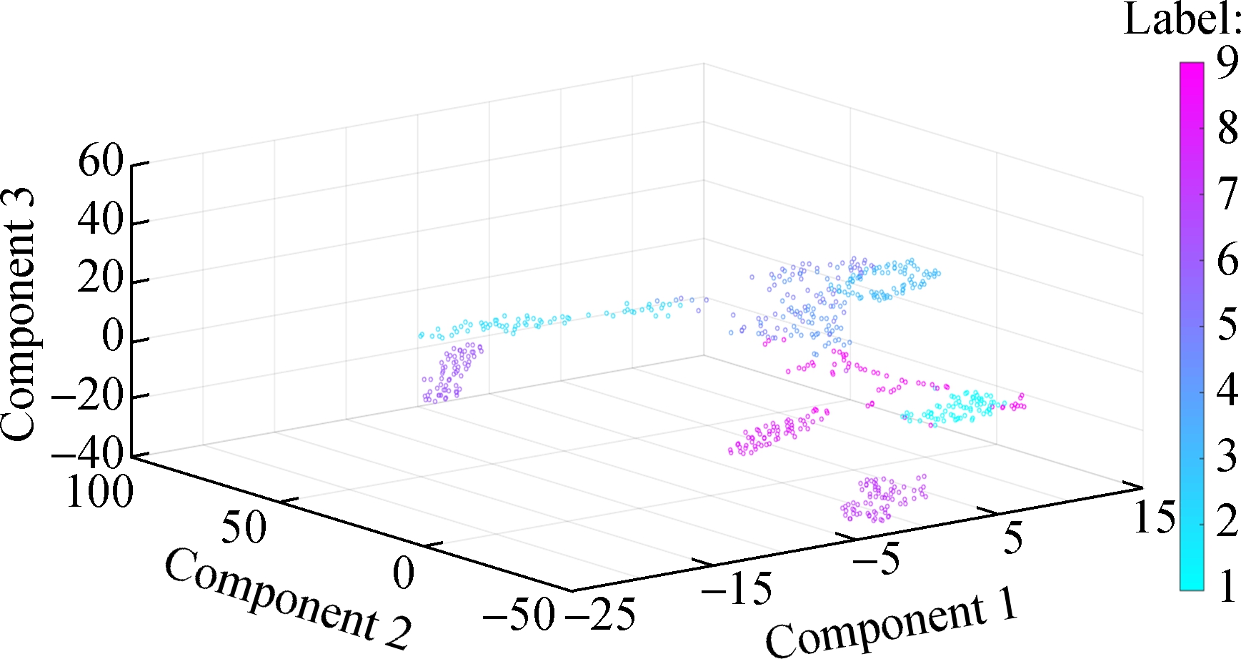
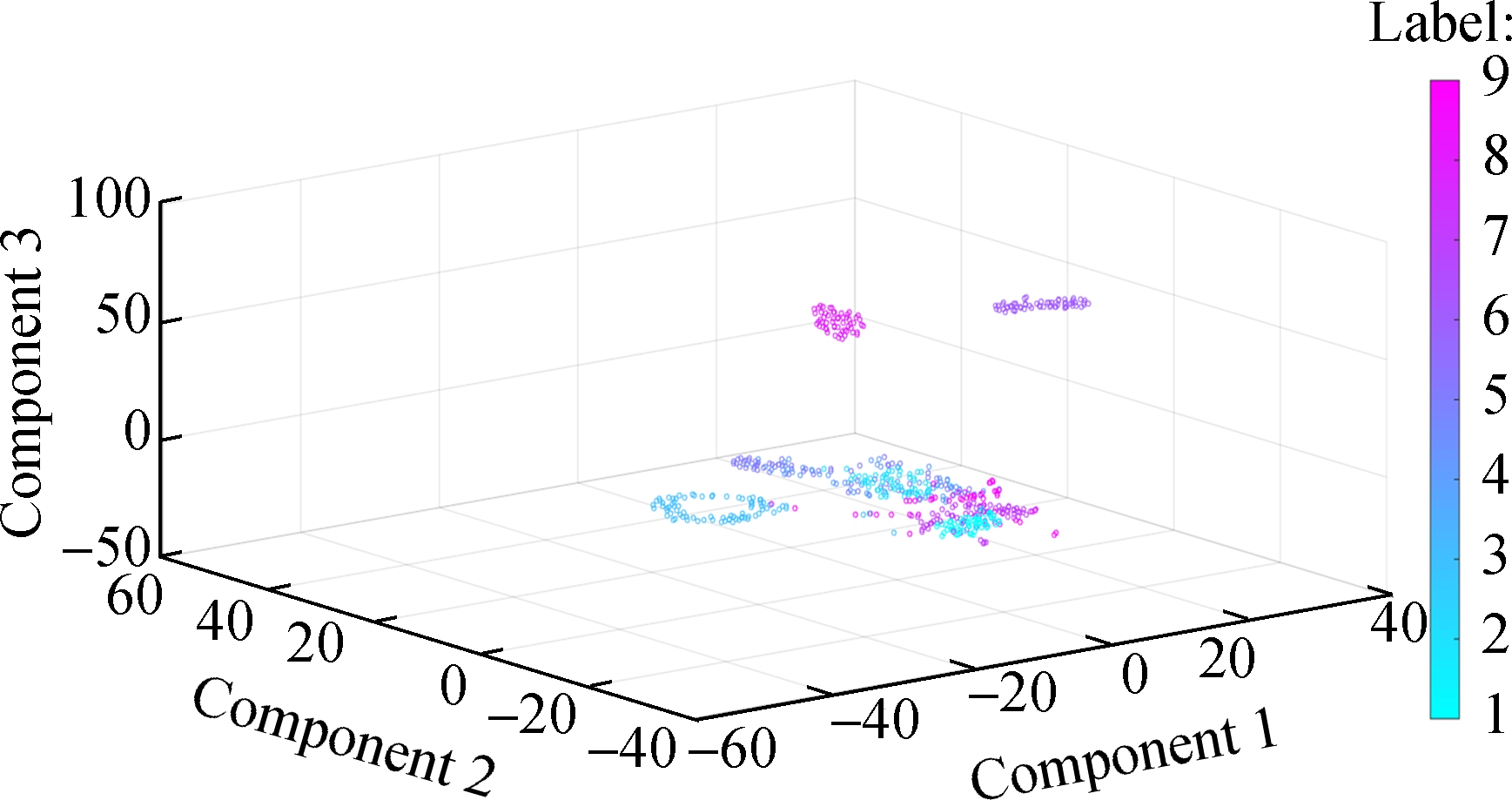
In order to visualize the differences between these methods, we use a technique called t-SNE[17]. It should be noted that we take the data length of 2 048 as an example of feature visualization for analysis. First, the principal component analysis(PCA) is used to reduce the high-dimensional data of the soft max layer to 3-D, and then the scatter plot for each test data is obtained. Fig.7(a) is the feature visualization of 2DCNN, Fig.7(b) is the visualization of 1DSCNN, and Fig.7(c) is the feature visualization of 1DLCNN. Through comparisons, it can be clearly seen that the separation phenomenon of different categories in Fig.7(c) is obvious, while the aliasing phenomenon occurs in the other two cases, which also demonstrates that the classification effect of 1DLCNN is optimal.
(a)
(b)

(c)
Fig.7 Feature visualization clustering of different methods. (a) 2DCNN; (b) 1DSCNN; (c) 1DLCNN
4 Conclusions
1) When using the one-dimensional large-kernel convolution neural network for fault diagnosis, an original one-dimensional vibration signal is directly inputted into the network without the expert experience. The diagnosis accuracy of this method is more accurate than that of the traditional fault diagnosis method.
2) The genetic algorithm can optimize the hyper-parameters of the network to obtain a set of optimal solutions. In this way, artificially selecting hyper-parameters can be avoided.
3) The high-dimensional features obtained by 1DSCNN and 2DCNN are confused, while 1DLCNN can separate different features clearly, so the one-dimensional large kernel is more advantageous when dealing with one-dimensional mechanical fault signals.
[1]Wu Z Y, Yuan H Q. Fault diagnosis of an engine with an ant colony support vector machine [J]. Journal of Vibration and Shock, 2009, 28(3): 83-86,201. DOI:10.13465/j.cnki.jvs.2009.03.037. (in Chinese)
[2]Hu Q, He Z J, Zhang Z S, et al. Fault diagnosis of rotating machinery based on improved wavelet package transform and SVMs ensemble[J].Mechanical Systems and Signal Processing, 2007, 21(2): 688-705. DOI:10.1016/j.ymssp.2006.01.007.
[3]Yuan S F, Chu F L. Support vector machines-based fault diagnosis for turbo-pump rotor[J].Mechanical Systems and Signal Processing, 2006, 20(4): 939-952. DOI:10.1016/j.ymssp.2005.09.006.
[4]Abbasion S, Rafsanjani A, Farshidianfar A, et al. Rolling element bearings multi-fault classification based on the wavelet denoising and support vector machine[J].Mechanical Systems and Signal Processing, 2007, 21(7): 2933-2945. DOI:10.1016/j.ymssp.2007.02.003.
[5]Han M H, Pan J L. A fault diagnosis method combined with LMD, sample entropy and energy ratio for roller bearings[J].Measurement, 2015, 76: 7-19. DOI:10.1016/j.measurement.2015.08.019.
[6]Wu G. Neural networks based fault diagnosis of rolling bearing [D]. Harbin: Harbin Institute of Technology, 2008.(in Chinese)
[7]You W, Shen C Q, Guo X J, et al. Bearing fault diagnosis using convolution neural network and support vector regression[C]// The 2017 International Conference on Mechanical Engineering and Control Automation. Nanjing, China, 2017: 6-11. DOI:10.12783/dtetr/icmeca2017/11904.
[8]Ding X X, He Q B. Energy-fluctuated multiscale feature learning with deep ConvNet for intelligent spindle bearing fault diagnosis[J].IEEE Transactions on Instrumentation and Measurement, 2017, 66(8): 1926-1935. DOI:10.1109/tim.2017.2674738.
[9]Chen Z Q, Li C, Sanchez R V. Gearbox fault identification and classification with convolutional neural networks[J].Shock and Vibration, 2015, 2015: 1-10. DOI:10.1155/2015/390134.
[10]Guo X J, Chen L, Shen C Q. Hierarchical adaptive deep convolution neural network and its application to bearing fault diagnosis[J].Measurement, 2016, 93: 490-502. DOI:10.1016/j.measurement.2016.07.054.
[11]Janssens O, Slavkovikj V, Vervisch B, et al. Convolutional neural network based fault detection for rotating machinery[J].Journal of Sound and Vibration, 2016, 377: 331-345. DOI:10.1016/j.jsv.2016.05.027.
[12]Wang F A, Jiang H K, Shao H D, et al. An adaptive deep convolutional neural network for rolling bearing fault diagnosis[J].Measurement Science and Technology, 2017, 28(9): 095005. DOI:10.1088/1361-6501/aa6e22.
[13]Wang X C, Shi F, Yu L, et al. 43 case studies of MATLAB neural network[M]. Beijing: Beihang University Press,2013:21-23.(in Chinese)
[14]Fu D P, Zhai Y, Yu Q M. Study on fault diagnosis of rolling bearing based on EMD and support vector machine[J].Machine Tool & Hydraulics, 2017, 45(11): 184-187. DOI:10.3969/j.issn.1001-3881.2017.11.042. (in Chinese)
[15]Ye R Z, Li W H. Fault diagnosis for bearings based on wavelet packet decomposition and BP neural network[J]. Bearing, 2012(10): 53-56. DOI:10.3969/j.issn.1000-3762.2012.10.019.(in Chinese)
[16]Pan Z R, Liu X, Qiao Z J. Intelligent fault diagnosis of rolling bearing based on wavelet packet energy and BP neural network [J]. Automation & Instrumentation, 2015(5): 82-84. DOI: 10.14016/j.cnki.1001-9227.2015.05.082. (in Chinese)
[17]Maaten L, Hinton G E. Visualizing data using t-SNE[J]. J Mach Learn Res, 2008, 9(3): 2579-2605.