In recent years, machine learning, deep learning and other methods in image recognition have experienced vigorous development. A variety of deep convolutional network models have made significant contributions to the field of image recognition, increasing the accuracy of image classification to new levels and achieving breakthroughs in all application areas. Deep learning is a branch of machine learning. It is a hierarchical model structure similar to that of the human brain. It extracts the characteristics of the input data from the bottom layer to the highest layer to establish a mapping relationship from the bottom signal to high-level semantics[1]. Today, it has become an inevitable trend for the Internet, big data, and artificial intelligence[2].
The CNN is the first successful learning algorithm for training multilayer network structures. CNNs use a gradient-based improved back-propagation algorithm to train the weights in the network. They implement a multilayer filtered network structure for deep learning and a global training algorithm combined with filters and classifiers, which reduces the complexity of the network model and the number of weights[3]. The CNN has achieved very good results in the image processing field[4]. After the development of the Alex-Net deep convolutional network model[5] for the ILSVRC-2012 fire in 2012, researchers continued to propose deep convolutions, such as the ALL-NET[6], ResNet-50[7], Inception-V3[8], and VGG-19[9] models. These models have achieved good performances in tasks such as image recognition, target detection, and semantic segmentation. The basis of these well-performing models is the need for sufficient training data to provide supervised training; therefore, the quality of the data sets is a fundamental factor that limits the training results of the deep convolutional network model.
Since data sets are usually developed manually, the quality of data sets is subjectively influenced by people. An important basis for judging the quality of a data set is the presence of noise images in each category. Elaborately produced open-source benchmark data sets, whose images of various categories are often represented by exact and true category semantics, can often achieve a high classification accuracy by using classification models applied to these data sets. Inspired by this, this paper starts from the perspective of image classification, uses noise data to train the classification model, and then uses the classification accuracy of the noiseless test set to reflect the impact of data set noise on the degraded performance of the deep convolutional network classification.
1 Data Set Noise Analysis
When the data set is in the production stage and the artificial subjective classification error occurs, it may add the remaining similar image in the data set to a certain category, or it may mistakenly add the image of an unrelated category to a specific category. The first operation introduces cross-category noise, and the second introduces random noise. For cross-category noise, the artificial standard category often mislabels multiple images in the same data class as a specific category. At this time, the noise concentrates on a certain class. In contrast, random noise has a wide range of irrelevant category images. For example, if the original image is randomly cropped during the training phase, the background containing no target is used as the specified data label. This background content often does not belong to any category. In the same data set, the proportion of noise data is usually uncertain, depending on the artificial subjective recognition experience and the proportion of the size in the target image.
To facilitate the analysis of noise data, this paper selects the reference data set as the data source and then samples the source data set to obtain different proportions of noise data. The subsequent experiments set multiple proportions of the noise control group for classification training. Finally, the normal test data is used to detect the classification accuracy. The idea of this analysis is as follows. After the benchmark data set is carefully annotated manually, the noise data is completely removed. At this time, artificially introducing certain types of noise can effectively analyze the effects of different noise types.
In this case, when simulating the convergence conditions of the training process, it is necessary to add noise to the training set and verification set during the noise analysis. The test set is used to reflect the performance degradation. Only test data with accurate classification can accurately reflect the real situation of the degradation of recognition performance under noise data. Therefore,noise should not be introduced into the test data in the analysis phase.
2 Experimental Data and Model Selection
This paper uses Cifar-10 and Cifar-100, which are two benchmark data sets, for classification testing. Both data sets add a specific proportion of random noise. To better judge the impact of cross-category noise on the quality of the data sets, a comparison was made here between the impact of single-category and multicategory cross-category noise on model recognition performance. Cifar-10 has 10 different categories. Furthermore, we tested its 10 categories separately. The Cifar-100 data set has 20 coarse labels, each with 5 fine labels. In this paper, among the 20 coarse labels, one fine label for each coarse label was arbitrarily selected as the final test object.
2.1 Introducing random noise
To introduce random noise images in the training set and validation set, the experiment randomly selected some images from ImageNet and scaled them to 32×32 and then added them to the training data and verification data proportionally.
2.2 Introducing cross-category noise
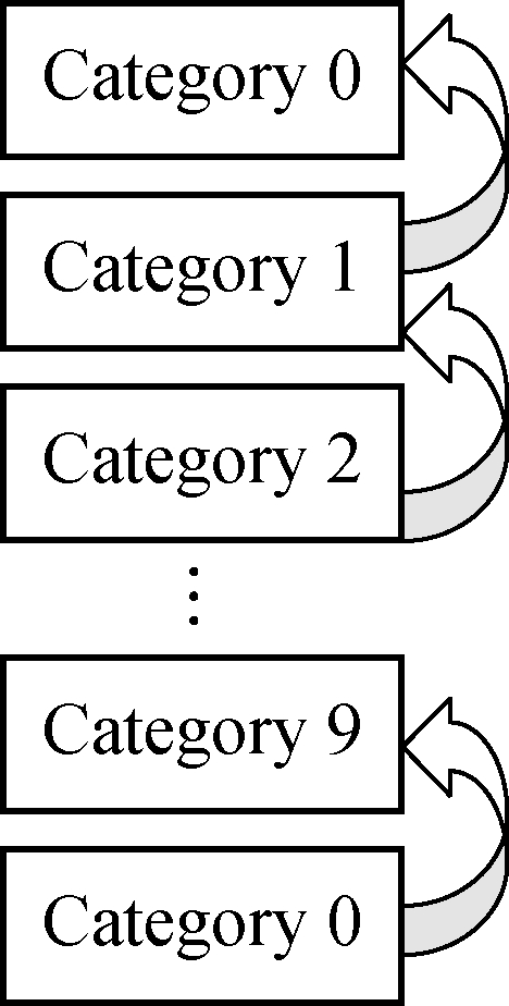
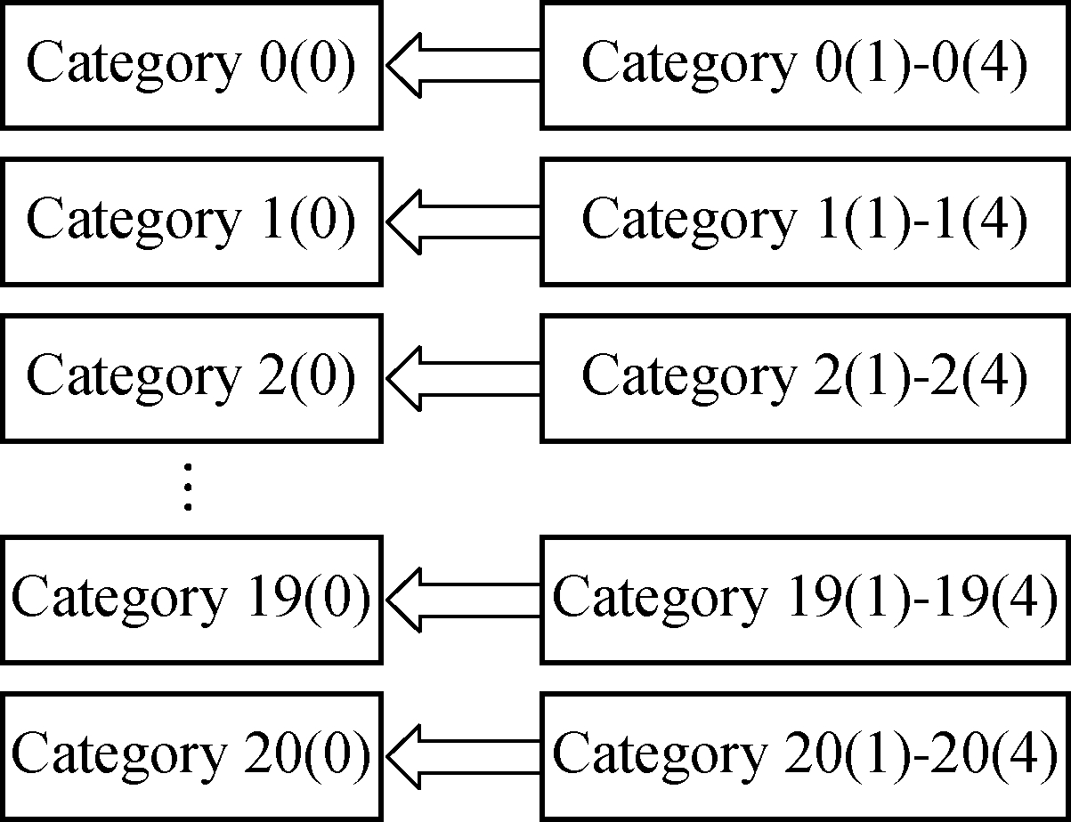
As shown in Fig.1, to introduce a cross-category noise image into the training data, in Cifar-10, the experiment directly added other categories to a specific category at a certain proportion. For Cifar-100, 20 coarse labels were separated from 100 categories, and 5 fine labels were separated from each coarse label. Among the 20 coarse labels, one fine-label was arbitrarily selected as a test object, and the other four fine labels were introduced as noise into the category at the same ratio. Therefore, the effect of introducing cross-category noise can be obtained. Here, (0) to (4) represent fine labels in every coarse label.
 (a)
(a)
(b)
Fig.1 Adding cross-category noise to Cifar-10 and Cifar-100.(a) Cifar-10;(b) Cifar-100>
2.3 Details of noise introduction
In this paper, four noise ratios are set to obtain reliable inferences from test data from multiple control groups. In both data sets, the proportion of noise images in the training set for each category is the same. In Cifar-10, the random noise and cross-category noise ratios are set to be 2.5%, 5%, 10%, and 20%, respectively. In Cifar-100, the ratio of random noise to total cross-category noise is the same as that of cifar-10. However, due to the introduction of four categories of noise, each noise ratio introduced should be the total cross-category noise ratio divided by four.
2.4 Model selection and its superiority
Classic convolutional neural networks consist of alternatively stacked convolutional layers and spatial pooling layers. The convolutional layers generate feature maps by linear convolutional filters followed by nonlinear activation functions (e.g., rectifier, sigmoid, and tanh). Using the linear rectifier as an example, the feature map can be calculated as
(1)
where (i,j) represents the pixel index in the feature map; xi,j is the input patch centered at location (i,j); k is used to index the channels of the feature map.
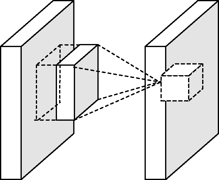
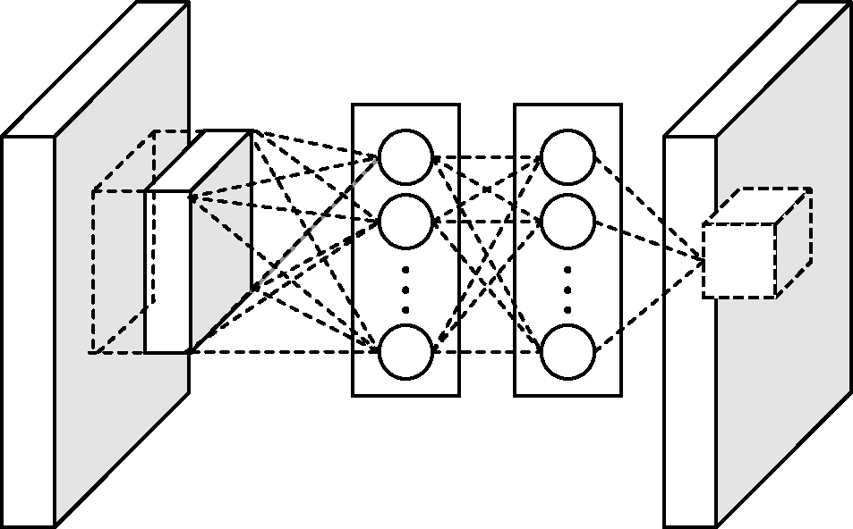
In fact, the high-level features of the CNN are actually a combination of low-level features through some kind of operation. According to this idea,the principle of NIN[10] is to perform more complex operations in each local receptive field and implement an improved algorithm for the convolutional layer: the MLP convolutional layer. Compared to the traditional convolutional layer process, the Mlpconv layer can be seen as a microlayer network in the local receptive field of each convolution. Fig.2 shows the difference between the linear convolution layer and the Mlpconv layer.
 (a)
(a)
(b)
Fig.2 The difference between the linear convolution layer and the Mlpconv layer.(a) Linear convolution layer; (b) Mlpconv layer
Using the micronetwork of the multilayer MLP, more complex operations are performed on each local receptive field neuron, and the nonlinearity is improved. The calculation process is as follows:
![]()
![]()
⋮![]()
(2)
where n is the number of layers in the multilayer perceptron. A rectified linear unit is used as the activation function in the multilayer perceptron.
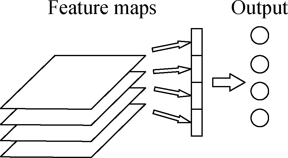
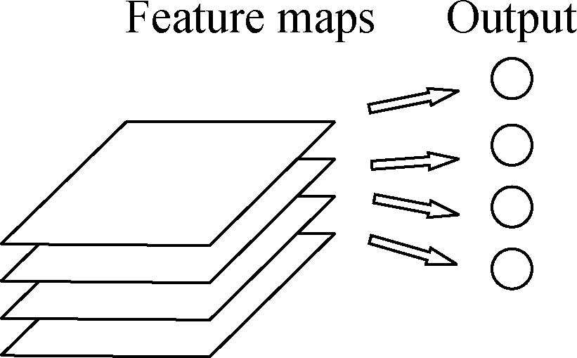
For the classification problem, unlike the fully connected layer in the traditional CNN,the principle of NIN is to use the mean pooling method to globally average the entire image of each feature map. In this way, you can obtain an output for each feature map, as shown in Fig.3. This can remove a large number of parameters for building a fully connected layer, which greatly reduce the network size and effectively avoid overfitting. On the other hand, it makes sense that each feature map is equivalent to an output feature.
 (a)
(a)
(b)
Fig.3 The difference between fully connected layers and global average pooling. (a) Fully connected layers; (b) Global average pooling>
Based on the above advantages, this paper uses NIN to classify categories. In fact, NIN, with a small number of parameters, has good performance with CIFAR-10 and CIFAR-100. The detailed settings are as follows. The model uses Relu activation to speed up model convergence. The loss term of the training optimization goal consists of the classification loss and L2 regularization term, where the weight of the L2 regularization term is 0.001. SGD is used to evaluate the loss function, and the learning rate is exponentially decayed. Otherwise, the dropout is set to be 0.5 to prevent overfitting. Finally, a softmax classifier is added to identify each category type. The number of iterations of the training process is 90.
3 Classification under Noise Conditions
In this experiment, Cifar-10 and Cifar-100 were trained using the noise settings above, and the NIN model was used to calculate the accuracy and average of each category on the test set.
3.1 Analysis of the average accuracy of each data set
Tab.1 shows the performance of the test set under the three training set training models by introducing various noise ratios. The leftmost AP value is the average accuracy rate predicted by the model trained using only normal graph data in the test set. The middle row of the AP values is the average accuracy under random noise. The rightmost AP value is the average accuracy under cross-category noise. Whether it is random noise or cross noise, the accuracy of model recognition decreases as the noise ratio increases. The former has less influence on the recognition ability of the model, and the latter has more significant effects.
In fact, if we take an extreme example, the effects of random noise and cross-category noise on the model become more apparent. Assuming that the model is perfect enough to achieve the correct classification of all categories, we can obtain the following conclusions:
If Rn=100% and Kn=1, then the original category is completely replaced by a new category,P1=1, A=0.
Otherwise, if Rn =100% and Kn=T, then the cross-category noise is approximated as random noise; therefore, the probability density function is
Tab.1 The average precision of classification of Cifar-10 and Cifar-100 in different noise situations

Noise ratio/%Normal images+No noiseNormal images+ Random noiseNormal images+ Cross-category noiseCifar-10Cifar-100Cifar-10Cifar-100Cifar-10Cifar-10000.8920.6580.8920.6580.8920.6582.50.8870.6680.8650.6630.8580.64450.8820.6470.8670.6320.8540.605100.8690.6500.8620.6460.8410.610200.8670.6420.8490.6150.8230.590
(3)
Thus, we can obtain PT≈1/T, A=1/T. Here, Rn is the rate of noise in the training data set; Kn is the number of cross-category noise types; P1 is the probability of adding cross-category noise; T is the number of training set images; PT is the probability of adding any one of T kinds of noise. The variable A is the recognition accuracy of the original category.
Obviously, the influence of cross-category noise is greater than that of random noise.
3.2 Methods to reduce the effects of cross-category noise
The greater the proportion of cross-category noise, the more significant the influence on the negative effects of the model. Therefore, reducing the proportion of cross-category noise effectively improves the recognition ability of the model. In Cifar-10, the training data is classified using a model that is initially trained to contain noise data. As shown in Tab.2, from the mixing matrix of the classification results, most of the cross-category noise categories can be effectively identified. For example, the 1 000 cross-category noise images whose labels are 0 in the training data have real labels of 1. A total of 909 of these images were judged to have labels of 1. Therefore, the screening of images that have been categorized as other categories in the training data can greatly reduce the cross-category noise ratio, and the recognition performance of the correspondingly retrained model is greatly improved.
Tab.2 The mixing matrix of the classification of cross-category noises in Cifar-10 before iterations

Category of training data with 20% noisePredicted category01234567890499090000305341459873517191753612176127655252513447631331641834378642414625112140595752913571541129700006152141047475825267164011001129615811120200104792797362023020301242
To obtain more accurate training data, we designed such an algorithm to separate interspersed cross-category noise as much as possible. By judging the data in the mixing matrix shown in Fig.9, if the recognition accuracy of the category can be improved, the images are reclassified. Then, the images are retrained, and the training data is classified to obtain a new mixing matrix. Here, we set the number of iterations to be 3. The specific flow chart is shown in Fig.4.
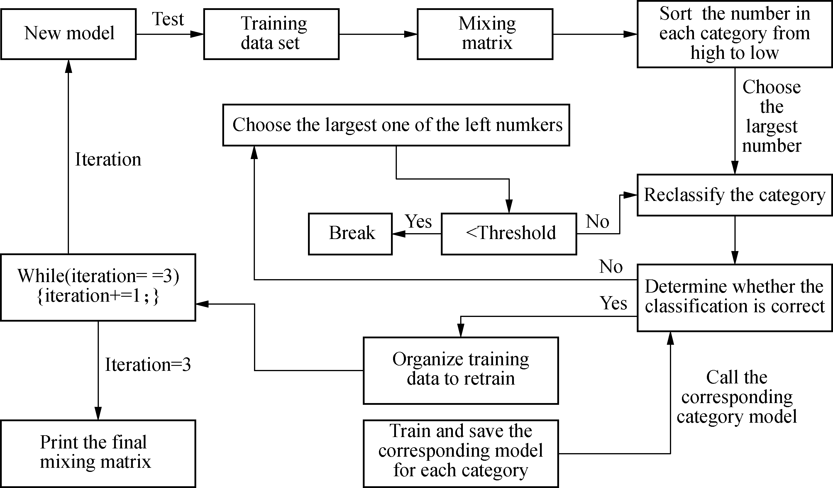
Fig.4 The algorithm flowchart for filtering of cross-category noise
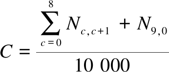
After three iterations, we can obtain a new mixing matrix, as shown in Tab.3. We find that the prediction of each introduced cross-category noise leaves only the noise category introduced and the original category. This shows that iterative screening does have a positive effect on correcting a wrong label. At the same time, it also shows that cross-category noise does affect the model’s extraction of the original category features, resulting in some images being incorrectly categorized. Of course, the more iterations there are, the less the noise of the data. After three iterations, the correction rate is 91.57% according to the following formula:
(4)
where C is the correction rate; c is the row label of the mixing matrix; N is the value of the current coordinate.
Tab.3 The mixing matrix for the classification of cross-category noise in Cifar-10 after three iterations
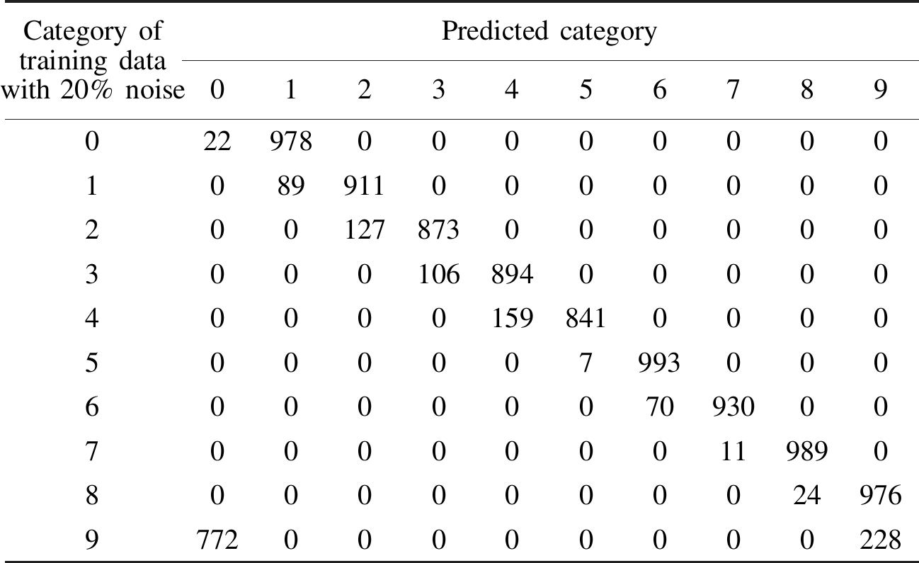
Category of training data with 20% noisePredicted category012345678902297800000000108991100000002001278730000003000106894000004000015984100005000007993000600000070930007000000011989080000000024976977200000000228
In Cifar-10, each category is mixed with a single category of noise. However, each fine label of Cifar-100 mixes into the other four categories of noise on the same coarse label. Similarly, we can also use the above model to obtain the mixing matrix, as shown in Tab.4.
Tab.4 The mixing matrix for the classification of cross-category noise in Cifar-100
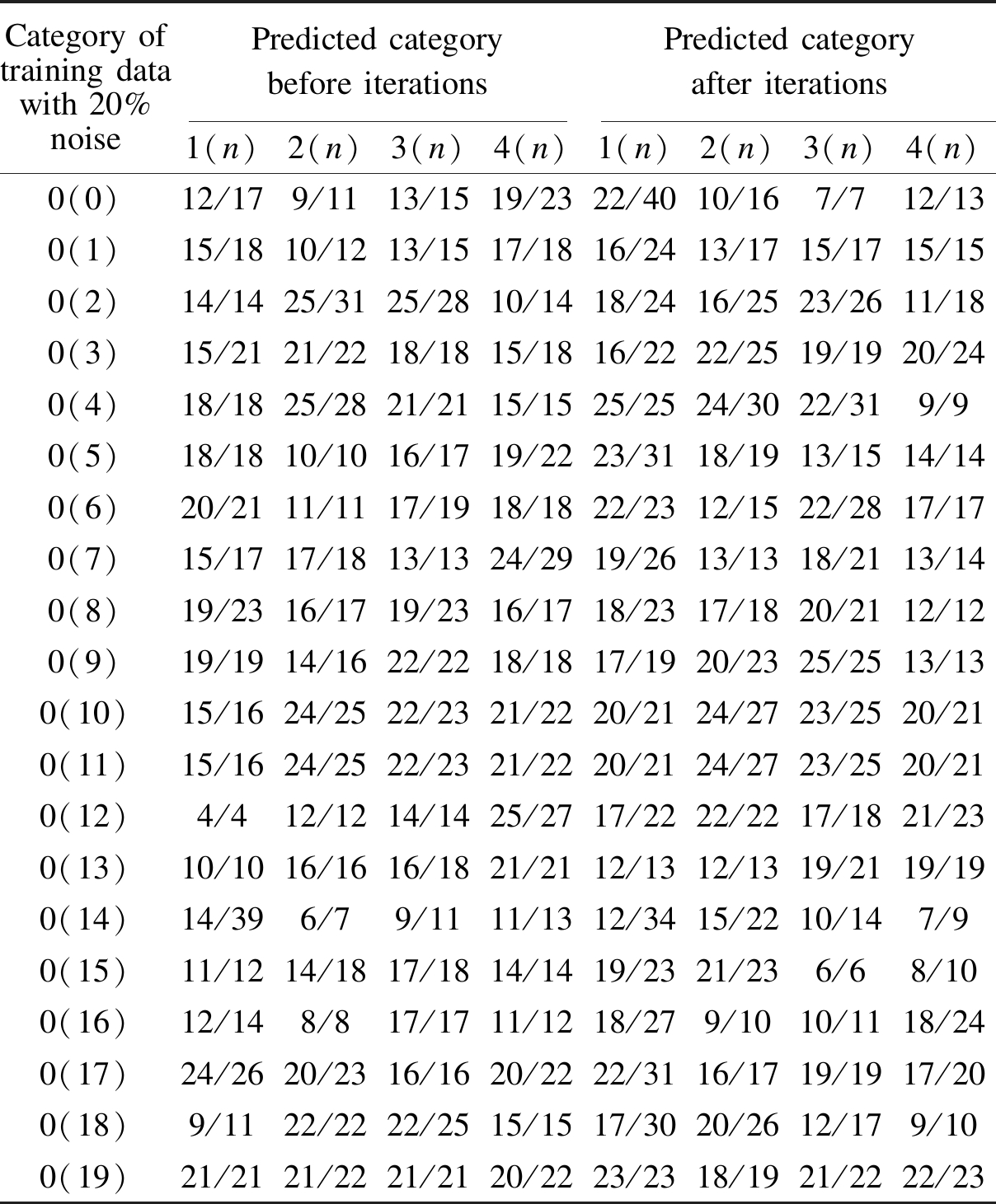
Category of training data with 20% noisePredicted categorybefore iterationsPredicted categoryafter iterations1(n)2(n)3(n)4(n)1(n)2(n)3(n)4(n)0(0)12/179/1113/1519/2322/4010/167/712/130(1)15/1810/1213/1517/1816/2413/1715/1715/150(2)14/1425/3125/2810/1418/2416/2523/2611/180(3)15/2121/2218/1815/1816/2222/2519/1920/240(4)18/1825/2821/2115/1525/2524/3022/319/90(5)18/1810/1016/1719/2223/3118/1913/1514/140(6)20/2111/1117/1918/1822/2312/1522/2817/170(7)15/1717/1813/1324/2919/2613/1318/2113/140(8)19/2316/1719/2316/1718/2317/1820/2112/120(9)19/1914/1622/2218/1817/1920/2325/2513/130(10)15/1624/2522/2321/2220/2124/2723/2520/210(11)15/1624/2522/2321/2220/2124/2723/2520/210(12)4/412/1214/1425/2717/2222/2217/1821/230(13)10/1016/1616/1821/2112/1312/1319/2119/190(14)14/396/79/1111/1312/3415/2210/147/90(15)11/1214/1817/1814/1419/2321/236/68/100(16)12/148/817/1711/1218/279/1010/1118/240(17)24/2620/2316/1620/2222/3116/1719/1917/200(18)9/1122/2222/2515/1517/3020/2612/179/100(19)21/2121/2221/2120/2223/2318/1921/2222/23
Notes: 0 (1) represents the fine label 0 in the coarse label 1. The rest is similar.17 in 12/17 represents the total amount of 1(0) predicted and corrected, but the correct number is only 12.The rest is similar.
As seen from Tab.4, this algorithm is actually very bad for data sets mixed into multiple categories of noise. Although it can correct the type of mixed noise to a certain extent, it mixes various types of noise into other categories, which causes the noise distribution to be more extensive. In other words, there is almost no completely correct category for the entire training data set. Therefore, this algorithm only has a significant effect on correcting data sets with a single category of noise. For a data set mixed into multiple types of noise, it becomes worse.
4 Conclusions
1) The recognition rate of each category in the data set has a different degree of reduction with increased noise ratio.
2) Compared with the introduction of random noise, the introduction of cross-category noise has a more significant influence on the recognition effect.
3) From the mixing matrix shown above, it can be seen that for a data set mixed into a single category, to reduce the influence of cross-level noise, the initial training model can be used to filter the cross-category noise in the training data so that the quality of the data set can be effectively improved. After filtering, the noise ratio of the data set can be significantly reduced. However, for a data set mixed into multiple categories of noise, the algorithm of this paper cannot improve its quality, which requires further research.
[1]Erhan D , Courville A, Bengio Y. Understanding representations learned in deep architectures, Technical Report 1355 [R]. Montreal, Canada: Universite de Montr’ eal, 2010.
[2]Hinton G E. Reducing the dimensionality of data with neural networks[J].Science, 2006, 313(5786): 504-507. DOI:10.1126/science.1127647.
[3]Krizhevsky A, Hinton G. Learning multiple layers of features from tiny images[R]. Toronto, Ontario, Canada: University of Toronto, 2009.
[4]Yu D, Deng L. Deep learning and its applications to signal and information processing [exploratory DSP][J]. IEEE Signal Processing Magazine, 2011, 28(1): 145-154. DOI:10.1109/msp.2010.939038.
[5]Krizhevsky A, Sutskever I, Hinton G E. ImageNet classification with deep convolutional neural networks[C]// International Conference on Neural Information Processing Systems. Curran Associates Inc, 2012:1-9.
[6]Springenberg J T, Dosovitskiy A, Brox T, et al. Striving for simplicity: The all convolutional net[J]. arXiv preprint arXiv:1412.6806, 2015.
[7]Zagoruyko S, Komodakis N. Wide residual networks[J]. arXiv preprint arXiv:1605.07146, 2016.
[8]Szegedy C, Vanhoucke V, Ioffe S, et al. Rethinking the inception architecture for computer vision[C]//Proceedings of the IEEE Conference on Computer Vision and Pattern Recognition. 2016: 2818-2826.
[9]Simonyan K, Zisserman A. Very deep convolutional networks for large-scale image recognition[J]. arXiv preprint arXiv:1409.1556, 2014.
[10]Lin M, Chen Q, Yan S. Network in network[J]. arXiv preprint arXiv:1312.4400, 2013.