Image restoration is a major subtopic in image science and has been extensively studied over the past decades. The purpose of image restoration is to reconstruct a high-quality image from its degraded observation. It is typically treated as an ill-posed linear inverse problem that can be generally formulated as
b=Hx+n
(1)
where b is the degraded observation; x is the desired true image; and n is Gaussian white noise with a zero mean. Note that H is a matrix representing a linear degradation operator.
To address the ill-posed nature of the image restoration problem, image prior knowledge is usually employed to regularize the solution of the following minimization problem:
(2)
where the first term is the data fidelity term and the second term Φ(x) is known as the regularization term, which regularizes the solution by enforcing certain prior constraints. In addition, λ>0 is the regularization parameter, which controls the balance between the fidelity and regularization terms.
How to select a good regularization term is an active area of research. Traditional regularization methods include Tikhonov regularization[1] and total variation (TV) regularization [2]. The total variation measure has been shown to be suitable for preserving sharp edges. Although TV regularization has been proven to be very useful in many applications, it is flawed in that it removes textures and creates staircase artifacts. Texture preserving methods such as sparse representations, non-local methods[3-5] and the deep convolutional neural network (CNN)-based method[6-7] have been introduced as image restoration approaches. Sparse regularization is a recent and successful method to solve image restoration problems[8-9]. Most sparse-based methods represent signals from a given dictionary and then process the coefficients of expansion individually. However, in addition to sparsity, signals may exhibit a “group sparsity” structure. Group sparsity is usually modeled by introducing a coupling between coefficients in the same structure set[10-12]. In the framework of variational formulation, this type of coupling may be introduced by a suitable regularization term[13]. In this study, we introduce a mixed norm regularization term, which enforces the sparsity on the LSD matrix of the restored image.
LSD is an important measure for the structural information of the image[14-15]. Through numerical experiments, we observed that the dynamic range of LSD decreases with an increase in noise intensity. Enforcing the sparsity of LSD matrix can efficiently equalize the LSD distribution. In this study, we examine the wavelet characterization of the LSD matrix of an image, and then propose a group sparse optimization model in the wavelet domain.
We describe the wavelet characterization of the LSD matrix, and then introduce the tree-structured group sparse model in the wavelet domain. Secondly, we give the solution of the proposed model based on different cases through the ADMM and FISTA techniques. Finally, some numerical experiments are presented to verify the potential of the proposed model.
1 Wavelet Characterization of LSD Matrix
In this study, an image is interpreted as a function defined on the unit square I=[0,1]2. Let Q be the collection of dyadic cubes contained in I.
(3)
where j=0,1,…;k=(k1,k2)∈Γj={0,1,…,2j-1}2.
Let φ and ψ be a univariate wavelet constructed out of Vj, which is an r-regular multiresolution approximation of L2(R2)with r≥1(for the exact conditions, see Ref.[16]). Two dimensional wavelets can be constructed by a tensor product
![]() ·ψε2(2jx2-k2)
·ψε2(2jx2-k2)
where j∈Ζ, k=(k1,k2)∈Ζ2,ε∈E=(ε1,ε2)2/{0,0} with εj=0 or 1,ψ0=φ, and ψ1=ψ.
One can easily construct periodic wavelets on L2(I) that can be used to decompose periodic function f on L2(I).
For a compactly supported wavelet ![]() we define its periodic version, which is still denoted here by
we define its periodic version, which is still denoted here by
For the wavelet decomposition of functions in L2(R2), we do not need to translate all of these periodic wavelets. On level j, we need only the translates k∈Γj.Because the translates of the scaling function form a partition of unity, we can obtain ![]() which is the characteristic function of I. The wavelet expansion for a function f∈L2(R2) is
which is the characteristic function of I. The wavelet expansion for a function f∈L2(R2) is
(4)
and the L2 norm of f can be characterized by wavelet coefficients:
(5)
In this subsection, we derive the wavelet characterization of the LSD matrix of f on dyadic region QJ,K. The LSD matrix is defined as
(6)
where J=0,1,…, and K=(K1,K2)∈ΓJ={0,1,…,2J-1}2 are the indices for characterizing the dyadic cube QJ,K defined in Eq.(3); ![]() is the mean of f on the dyadic region QJ,K;QJ,K denotes the volume of QJ,K and QJ,K=22J.
is the mean of f on the dyadic region QJ,K;QJ,K denotes the volume of QJ,K and QJ,K=22J.
The LSD matrix characterizes the local oscillating property of the image. Different components of an image may have different LSD. In a homogenous region, the LSD is rather small, while in an edge and texture region, the LSD becomes large. Generally, the LSD of noise is much smaller than that of texture. Thus, LSD is often used to separate homogeneous and textured regions in natural image denoising.
In Ref.[17], we derive the discrete wavelet characterization of the LSD matrix, which can be described by the following theorem.
Theorem 1 The LSD matrix of f on dyadic region QJ,K can be characterized by wavelet coefficients as follows:
![]()
![]()
(7)
Proof Let C(QJ,K) denote the mean value of f(x) on QJ,K,then
![]()
![]()
(8)
![]() ·
·![]()
C(QJ,K)·2J·![]() ·2J·2-2J=
·2J·2-2J=![]()
(9)
We write f(x) as f(x)=f1(x)+f2(x)+C(QJ,K), where
(10)
By Eq.(9), we can obtain
(11)
Since f2(x)=0 if x∈QJ,K, and the support of ![]() is contained in QJ,K, we have
is contained in QJ,K, we have ![]() Thus,
Thus,
(12)
Then,
![]()
![]()
![]()
(13)
Then, we can obtain
2 Group Sparse Model in The Wavelet Domain
Let f∈Rm×n be an image. We assume that f has the multi-scale wavelet expansion as indicated in Eq.(4). Then, the support of ![]() where QJ,K=sup
where QJ,K=sup ![]() As indicated in Eq.(4), f is decomposed into low-frequency component and high-frequency component, which are denoted by fL and fH, respectively.
As indicated in Eq.(4), f is decomposed into low-frequency component and high-frequency component, which are denoted by fL and fH, respectively.
For fixed scale J, let GK={(j,k,ε):Qj,k⊆QJ,K,j≥J,k⊆Γj,ε∈E} denote the index set. Then, ![]() ·{αGK}K∈ΓJ forms a non-overlapping partition of all high-frequency coefficients. Note that the wavelet coefficients in each group {αGK}K∈ΓJ have a parent-child relationship with the tree structure (see Fig.1). With this grouping strategy, we can rewrite the LSD matrix PJ,K as follows:
·{αGK}K∈ΓJ forms a non-overlapping partition of all high-frequency coefficients. Note that the wavelet coefficients in each group {αGK}K∈ΓJ have a parent-child relationship with the tree structure (see Fig.1). With this grouping strategy, we can rewrite the LSD matrix PJ,K as follows:
PJ,K(f)=2J‖αGK‖2 K∈ΓJ
(14)
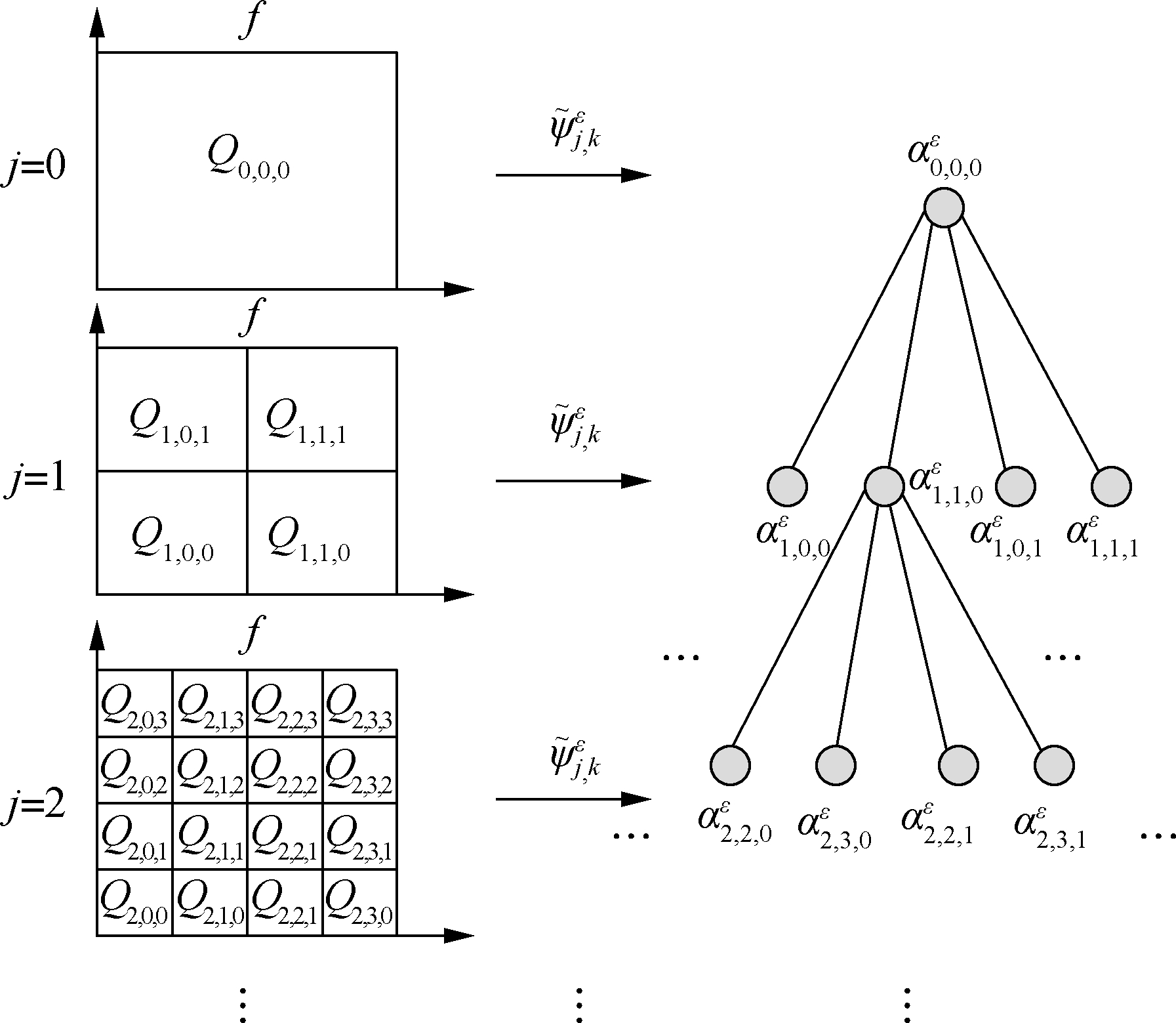
Fig.1 Tree-structured wavelet coefficients
In this study, we introduce the prior that the LSD matrix PJ,K is sparse. This can be obtained by minimizing the l1 norm of the LSD matrix. In other words, we use the following weighted l2,1 norm as a regularizer:
(15)
where ωK are weights associated with each group. Properly choosing weights may result in improved recovery performance. In this study, we choose ωK as
(16)
The mixed norm in Eq.(15) explicitly introduces the coupling between wavelet coefficients instead of the usual independence assumption of lp norm sparse optimization problems. Thus, we consider the following regression problem to recover the group sparse solution:
(17)
where bH is the high-frequency component of observed image b, and W is the wavelet transform. ωK controls the group sparsity level adaptively. While the image regions are dominated by texture and edges,PJ,K is relatively large and ωK is relatively small. Then, the wavelet coefficients group αGK is less penalized such that the edges and texture are well preserved during denoising. Conversely, in homogeneous image regions, PJ,K is relatively small and ωK is relatively large. Then, αGK has more intense shrinkage to enhance the denoising process.
Because most of the noise is concentrated in the high-frequency component, we must only recover the high-frequency component of the image. If α* is the solution of model (17), then the final restored image is b*=WTα*+bL, where bL is the low-frequency component of the observed image.
Our intent is not to seek a state-of-the-art denoising method, but rather to investigate the sparsity of LSD as signal priors and compare it to the TV-based, frame-based and non-local mean methods.
3 Solution of the Proposed Model
We apply the ADMM to solve model (17) when H is identity and WT is a linear operator (for the ADMM algorithm, see Ref.[18]). To accomplish this, we introduce an auxiliary variable and transform model (17) into an equivalent form:
(18)
s.t. Z=α
(19)
The augmented Lagrangian problem takes the form:
![]()
![]()
(20)
where μ>0 is a multiplier and β1 is a penalty parameter. We then apply the ADMM to minimize the Lagrangian problem alternately with respect to Z and α.
The α subproblem is given by
(21)
Note that(21) is a convex quadratic problem. Therefore, its solution is
(22)
For the Z subproblem, it is reduced to minimize (20) with respect to Z:
(23)
By simple manipulation,(23) is equivalent to the following problem:
(24)
This can be solved by group-wise soft shrinkage:
(25)
The multiplier μ is updated by
μ←μ+τ(Z-α)
(26)
where τ is the step length. In summary, we obtain the algorithm for solving model (17) by ADMM as shown in the following:
Algorithm 1 ADMM for model (17) when H is identity
Input: bH,Z0, μ0, β1,β2, τ.
Iteration:For k=1,2,…, until a stopping criterion is reached,
![]()
![]()
μk=μk-1+τ(Zk-αk)
Output: αk.
Note that regularizer ‖·‖lw,2,1 is non-smooth but convex, whereas the fidelity term is smooth and convex. Thus, in the following we apply the iterative shrinkage-thresholding algorithm (ISTA) to solve the general case of model (17). The general step of ISTA is described as
αk+1=Proxtkg(αk-tkWHT(HWTαk-bH))
(27)
where g(·)=λ‖·‖lw,2,1 is the mixed norm functional proposed in (15), and Prox is the proximal operator. The proximal algorithm is an efficient tool for non-smooth minimization problems. In proximal algorithms, the base operation is to evaluate the proximal operator of a function, which involves solving a small convex optimization problem. The proximal operator is defined by
Therefore, the Proxtkg operation in (27) can be expressed as
(28)
The Prox operation can be easily solved by group-wise shrinkage, that is
Proxtkg(x)=GShink(x,λtkω)
(29)
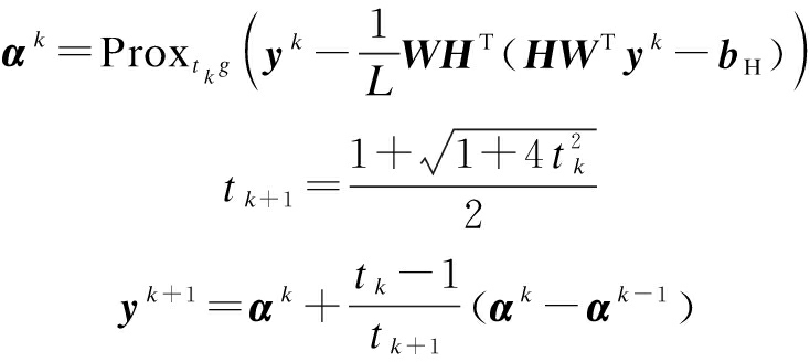
Although ISTA has the advantage of simplicity, it has also been recognized to be a slow method. The fast iterative shrinkage thresholding algorithm (FISTA) is the accelerated version of ISTA[19]. It not only preserves the computational simplicity, but also exhibits a significantly faster convergence rate than standard gradient-based methods. Algorithm 2 summarizes the FISTA for solving model (17), which is described as follows:
Algorithm 2 FISTA for model (17)
Input: bH, α0=0,t1=1,y1=α0,L,λ.
Iteration: For k=1,2,…, until a stopping criterion is reached,
Output:αk.
4 Experiments
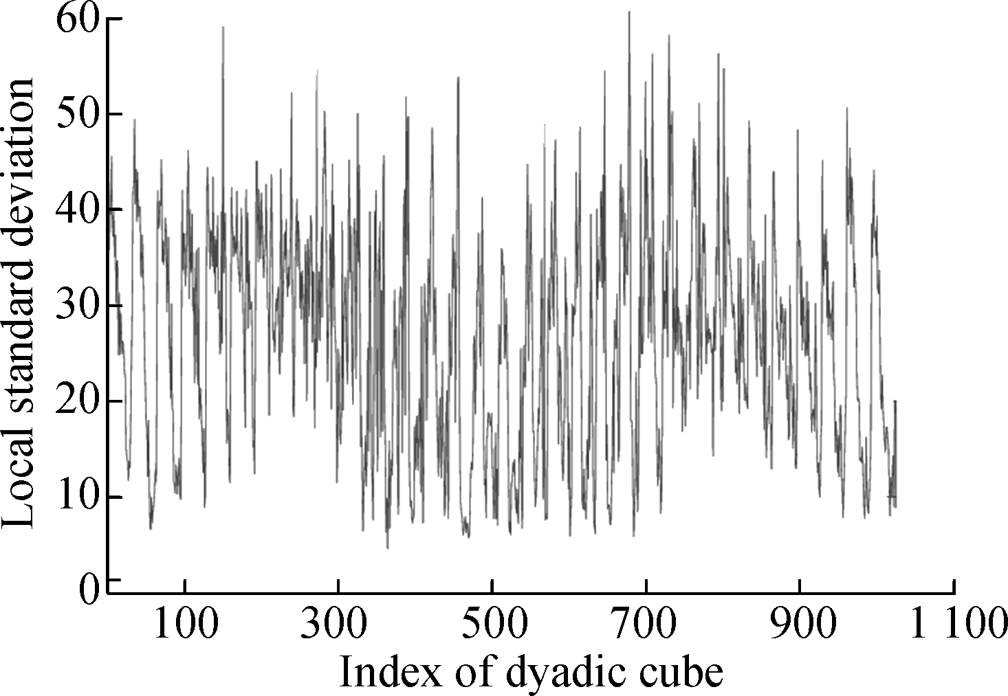
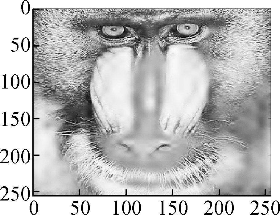
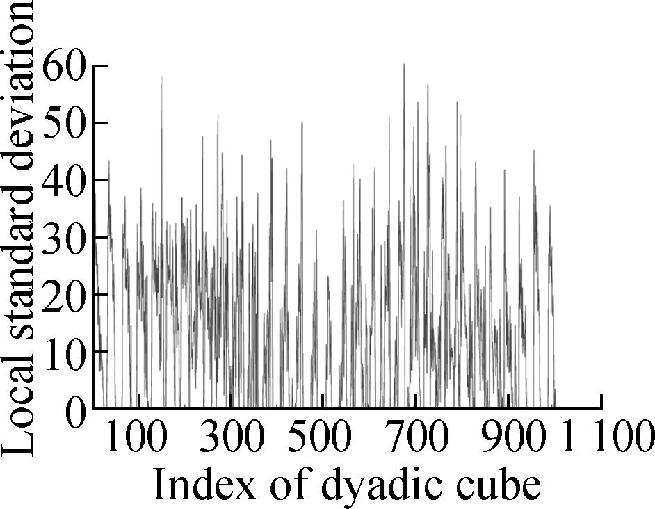
In this section, we present various experiments to show the performance of the proposed method for image denoising. In all the experiments, we chose the periodic “sym4” wavelet and scale J=6. First, we describe the group sparse approximation performance of the proposed model based on a noiseless case, as shown in Figs.2 and 3. Fig.2(a) shows the original “Baboon” image and Fig.2(b) shows the plot of the vectorization of its LSD matrix. The vectorization is obtained by stacking the columns of the LSD matrix on top of one another. From the plot of vectorized LSD matrix, we can easily observe its sparsity.
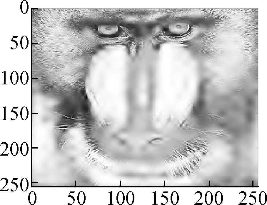
Figs.3 (a) to (d) show the group sparse approximation with parameters β2=0.001, 0.002, 0.004 and 0.007, respectively. Figs.3(e) to (h) show the corresponding vectorized LSD matrix. There are a total of 1 024 groups of wavelet coefficients, and the percentages of non-zero groups of the approximation image with different parameters are listed in Tab.1.
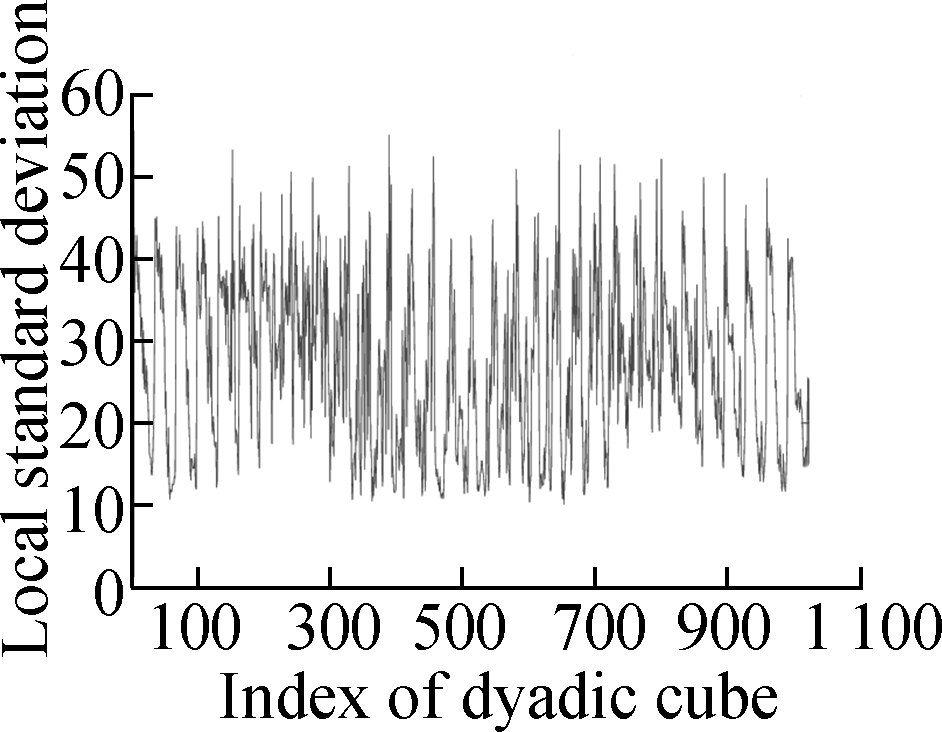
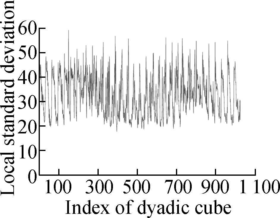
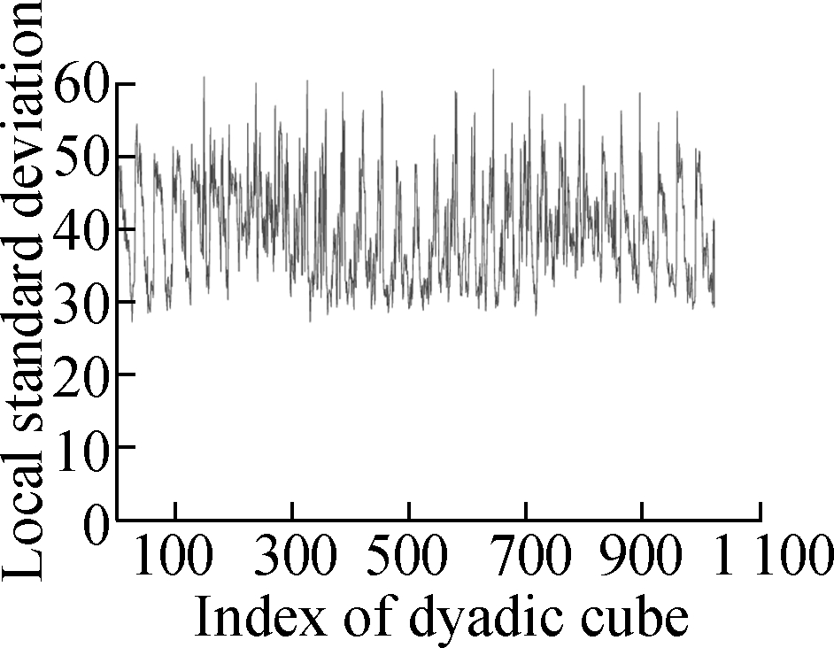
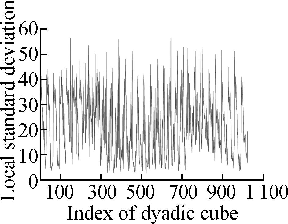
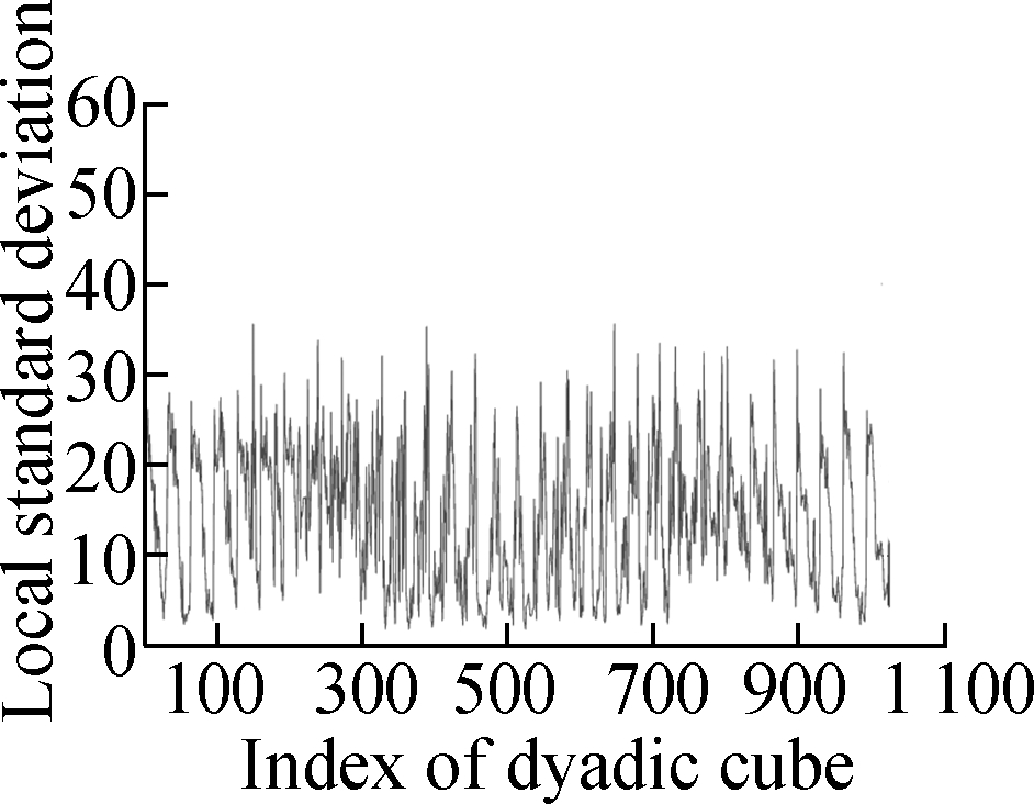
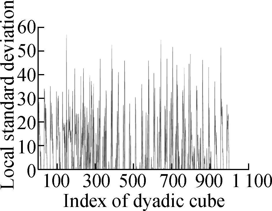
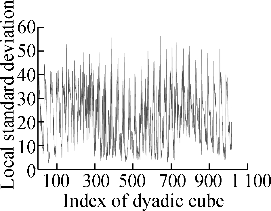
Fig.4 shows the evolution of the LSD matrix along with the noise level. Figs.4(a) to (c) show the noisy Baboon images degraded by three levels of Gaussian noise with a mean of zero and standard deviations of 10, 20, and 30, respectively. Figs.4(d) to (f) show the corresponding vectorized LSD matrix. We can see that the dynamic range of the LSD matrix becomes increasingly narrow with each increase in the standard deviation. The dynamic range of the LSD matrix is defined as We apply the ADMM algorithm to equalize the LSD matrix of the noisy Baboon image (σ=15). In Fig.5 and Tab.2, we present the experimental results to show how parameters β1 and β2 affect the group sparsity and the range of the LSD matrix. We can see that parameterβ2 controls the group sparsity of the solution and parameter β1 controls the range of the LSD matrix. The group sparsity can be measured by the group sparsity rate ρ, which is the percentage of the non-zero groups.

(a)
(b)
Fig.2 Test image Baboon and the corresponding LSD matrix. (a) Original 512 × 512 Baboon image; (b) Vectorized LSD matrix of (a)


(a) (b) (c) (d)



(e) (f) (g) (h)
Fig.3 Group sparse approximation result and the corresponding vectorized LSD matrix on noiseless image Baboon (β1=0.2). (a) β2=0.001; (b) β2=0.002; (c) β2=0.004; (d) β2=0.007; (e) Vectorized LSD matrix of (a); (f) Vectorized LSD matrix of (b); (g) Vectorized LSD matrix of (c); (h) Vectorized LSD matrix of (d)
Tab.1 Group sparse approximation performance with different parameters

Parameter β2Number of non-zero groupsPercentage/%0.00188486.330.00258757.320.00434833.980.00718417.97


(a) (b) (c)
(d) (e) (f)
Fig.4 Evolution of the LSD matrix along with the noise level. (a) Noisy image with noise std of 10; (b) Noisy image with noise std of 20; (c) Noisy images with noise std of 30; (d) Vectorized LSD matrix of (a); (e) Vectorized LSD matrix of (b); (f) Vectorized LSD matrix of (c)
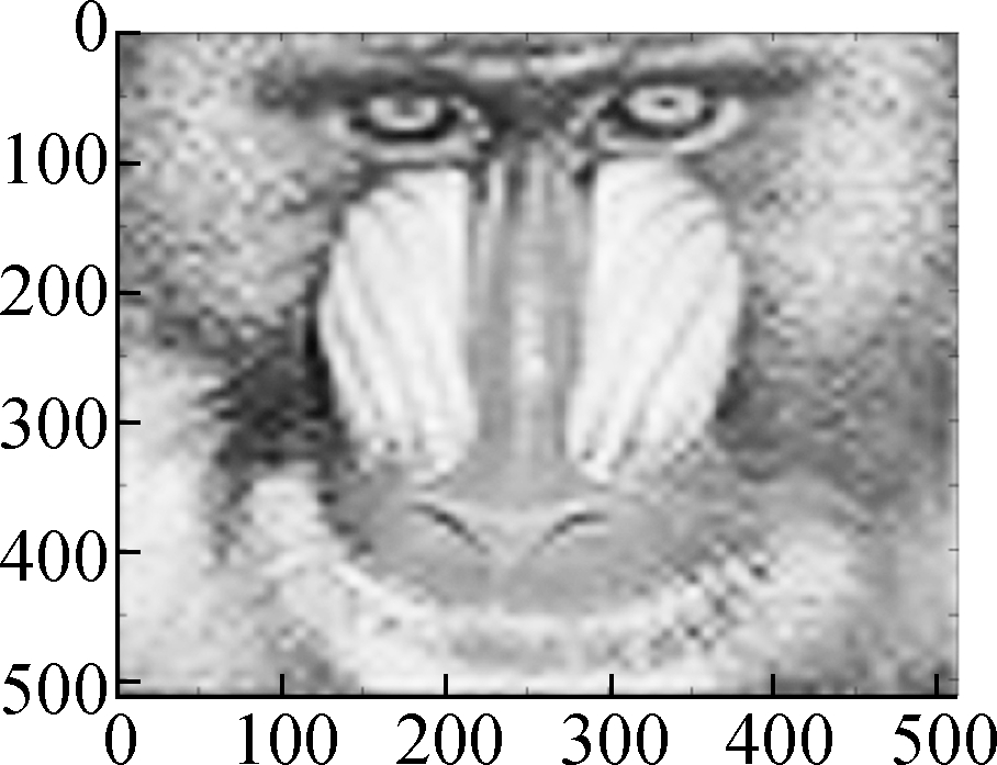
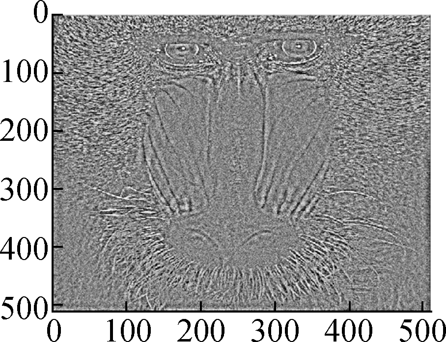
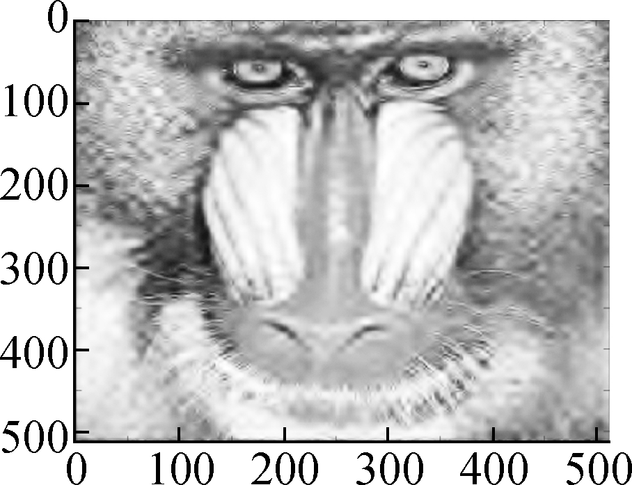
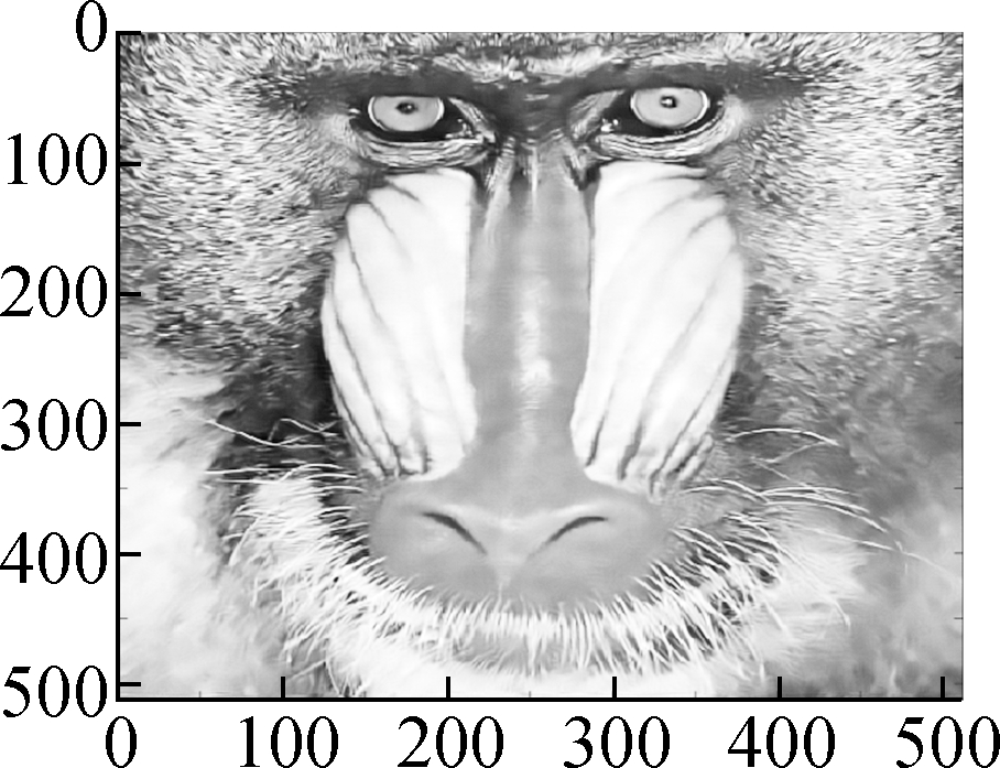
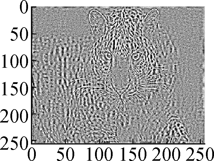
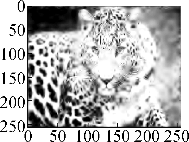
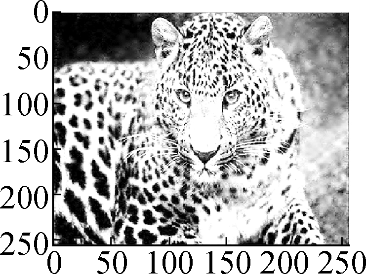
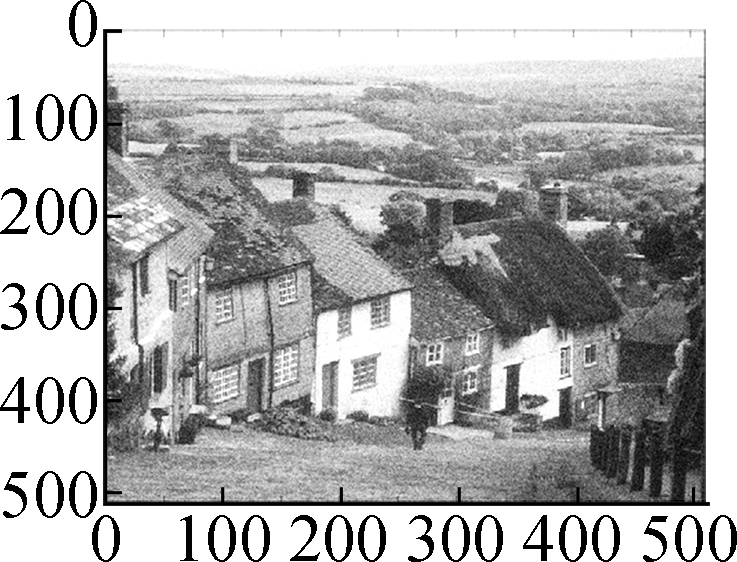
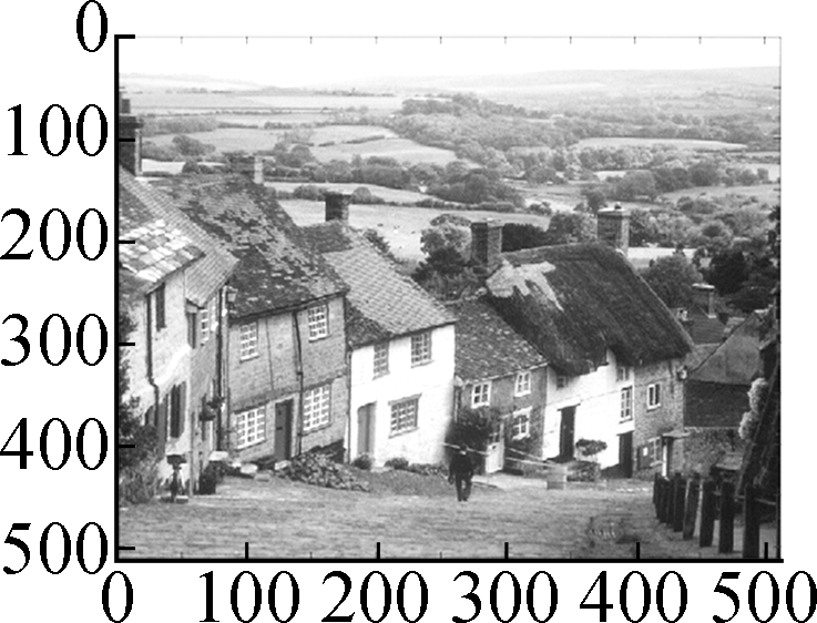
In Figs.6 to 8 and Tab.3, the denoising performance of Algorithm 1 is compared with that of the wavelet shrinkage model, TV model, balanced frame-based model[8], and non-local mean model[5]. We can see that the proposed model outperforms the wavelet shrinkage model and frame-based model, and achieves a competitive performance as compared with the TV model and non-local mean model.
Tab.2 Impact of parameters β1 and β2 on ρ and R
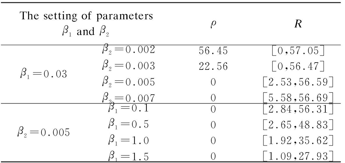
The setting of parameters β1 and β2ρRβ1=0.03β2=0.002β2=0.003β2=0.005β2=0.00756.4522.5600[0,57.05][0,56.47][2.53,56.59][5.58,56.69]β2=0.005β1=0.1β1=0.5β1=1.0β1=1.50000[2.84,56.31][2.65,48.83][1.92,35.62][1.09,27.93]


(a) (b) (c) (d)


(e) (f) (g) (h)
Fig.5 Performance of parameters β1 and β2 for controlling ρ and R. (a) β1=0.1,β2=0.005; (b) β1=0.5,β2=0.005; (c) β1= 1,β2=0.005; (d) β1=1.5,β2=0.005;(e) β1=0.03,β2=0.002; (f) β1=0.03,β2=0.003; (g) β1=0.03,β2=0.005; (h) β1=0.03,β2=0.007
Tab.3 Comparisons of PSNR performance with different models

ModelHill(σ=10)House(σ=10)Parrot(σ=15)Leopard(σ=15)Baboon(σ=15)Barbara(σ=20)Man(σ=20)Soft shrinkage 26.6226.4523.6417.9321.1823.1224.98Frame28.0930.4025.8723.7422.0524.3126.74TV29.9331.7328.6125.7826.0326.3229.14Nonlocal mean30.1232.4129.1925.4026.7730.3629.16Proposed model30.7532.3429.0526.3626.8226.8628.90

(a) (b) (c) (d)


(e) (f) (g) (h)
Fig.6 Comparison of denoising results by different models on the Baboon image (noise standard deviation σ=15).(a) Low frequency component bL by wavelet decomposition;(b) High frequency component bH by wavelet decomposition; (c) Restored high frequency by Algorithm 1; (d) Restored image by soft shrinkage model; (e) Restored image by balanced frame-based model; (f) Restored image by TV model; (g) Restored image by non-local mean model; (h) Restored image by Algorithm 1

(a)

(b)

(c)
(d)

(e)
(f)

(g)

(h)
(i)

(j)
Fig.7 Comparison of denoising results by different models on the Leopard image (noise standard deviation σ=15). (a) Original image; (b) Noisy version; (c) Low frequency bL by wavelet decomposition; (d) High frequency bH by wavelet decomposition; (e) Restored high frequency by Algorithm 1; (f) Restored image by soft shrinkage model; (g) Restored image by balanced frame-based model; (h) Restored image by TV model; (i) Restored image by non-local mean model; (j) Restored image by Algorithm 1
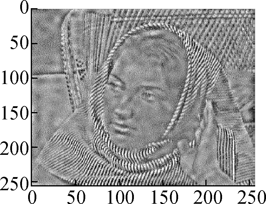
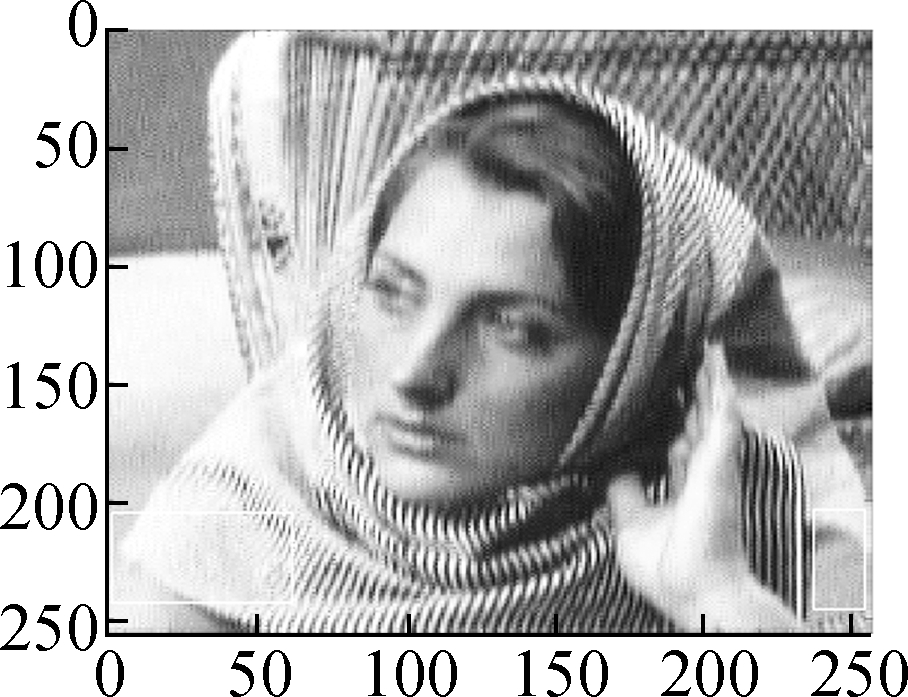
Fig.9 shows the results of Algorithm 2 on the woman image. The test image is contaminated by salt and pepper noise with noise intensity d=10%. After wavelet decomposition, most of the noises are concentrated in the high frequency component, which can be seen in Fig.9(c). Fig.9(d) shows the restored high-frequency component by the proposed model. One can see that most of the noises are removed and the textures are well preserved. Figs.9(e) to (g) compare the restored image by our method with that by the balanced frame-based method and non-local mean method. Particularly in the tagged region, we can see that the proposed method preserves more textures and achieves a better subjective visual effect.

(a)
(b)
(c)

(d)

(e)

(f)

(g)

(h)
(i)

(j)
Fig.8 Comparison of denoising results by different models on the Hill image (noise standard deviation σ = 10). (a) Original image; (b) Noisy version; (c) Low frequency component bL by wavelet decomposition; (d) High frequency component bH by wavelet decomposition; (e) Restored high frequency component by Algorithm 1; (f) Restored image by soft shrinkage model; (g) Restored image by balanced frame based model; (h) Restored image by TV model; (i) Restored image by non-local mean model; (j) Restored image by Algorithm 1


(a) (b) (c) (d)


(e) (f) (g)
Fig.9 Salt and pepper noise removal by Algorithm 2. (a) Original image (256×256); (b) Image contaminated by salt and pepper noise (noise intensity d=10%) ; (c) High-frequency component of (b); (d) Restored high-frequency component; (e) Restored image by balanced frame-based model; (f) Restored image by the non-local mean model; (g) Restored image by Algorithm 2
5 Conclusions
1) Based on the wavelet characterization of the LSD, we find that the l1 norm of the LSD matrix is equivalent to a l2,1 mixed norm of the wavelet coefficients. This mixed norm introduces a coupling between wavelet coefficients and determines a variable group scheme.
2) We find that enforcing the sparsity of the LSD can efficiently equalize the LSD distribution. Thus, we propose a novel group sparse optimization model in the wavelet domain for image denoising. Encoding the group information in addition to sparsity leads to better signal feature selection.
3) The group sparse optimization problem is more difficult to solve than the conventional l1 norm regularized problem. We applied the ADMM and FISTA to solve the group sparse model efficiently based on different cases.
4) Several experiments reveal that the proposed group sparse model outperforms traditional wavelet-based model and frame-based model, and has competitive performance with TV and non-local mean image restoration models.
[1] Tikhonov A N. Regularization of incorrectly posed problems [J]. Soviet Mathematics Doklady, 1963, 4: 1624-1627.
[2] Rudin L I, Osher S, Fatemi E. Nonlinear total variation based noise removal algorithms[J].Physica D: Nonlinear Phenomena, 1992, 60(1/2/3/4): 259-268. DOI:10.1016/0167-2789(92)90242-f.
[3] Buades A, Coll B, Morel J M. Nonlocal image and movie denoising[J].International Journal of Computer Vision, 2008, 76(2): 123-139. DOI:10.1007/s11263-007-0052-1.
[4] Ding D, Ram S, Rodriguez J J. Image inpainting using nonlocal texture matching and nonlinear filtering[J].IEEE Transactions on Image Processing, 2019, 28(4): 1705-1719. DOI:10.1109/tip.2018.2880681.
[5] Wang W, Li F, Ng M K. Structural similarity-based nonlocal variational models for image restoration[J].IEEE Transactions on Image Processing, 2019, 28(9): 4260-4272. DOI:10.1109/tip.2019.2906491.
[6] Zhang K, Zuo W, Chen Y J, et al. Beyond a Gaussian denoiser: Residual learning of deep CNN for image denoising[J].IEEE Transactions on Image Processing, 2017, 26(7): 3142-3155. DOI:10.1109/tip.2017.2662206.
[7] Jin K H, McCann M T, Froustey E, et al. Deep convolutional neural network for inverse problems in imaging[J].IEEE Transactions on Image Processing, 2017, 26(9): 4509-4522. DOI:10.1109/tip.2017.2713099.
[8] Starck J L, Elad M, Donoho D L. Image decomposition via the combination of sparse representations and a variational approach[J].IEEE Transactions on Image Processing, 2005, 14(10): 1570-1582. DOI:10.1109/tip.2005.852206.
[9] Cai J F, Osher S, Shen Z. Split bregman methods and frame based image restoration[J].Multiscale Modeling & Simulation, 2010, 8(2): 337-369. DOI:10.1137/090753504.
[10] Dong W S, Shi G M, Ma Y, et al. Image restoration via simultaneous sparse coding: Where structured sparsity meets Gaussian scale mixture[J].International Journal of Computer Vision, 2015, 114(2/3): 217-232. DOI:10.1007/s11263-015-0808-y.
[11] Zhang L, Zuo W. Image restoration: From sparse and low-rank priors to deep priors[J].IEEE Signal Processing Magazine, 2017, 34(5): 172-179. DOI:10.1109/msp.2017.2717489.
[12] Zhang J, Zhao D, Gao W. Group-based sparse representation for image restoration[J].IEEE Transactions on Image Processing, 2014, 23(8): 3336-3351. DOI:10.1109/tip.2014.2323127.
[13] Kowalski M. Sparse regression using mixed norms[J].Applied and Computational Harmonic Analysis, 2009, 27(3): 303-324. DOI:10.1016/j.acha.2009.05.006.
[14] Yang J Q, Zhu G P, Shi Y Q. Analyzing the effect of JPEG compression on local variance of image intensity[J].IEEE Transactions on Image Processing, 2016, 25(6): 2647-2656. DOI:10.1109/tip.2016.2553521.
[15] Li Z G, Zeng L, Xu Y F, et al. Level set method for image segmentation based on local variance and improved intensity inhomogeneity model[J].IET Image Processing, 2016, 10(12): 1007-1016. DOI:10.1049/iet-ipr.2016.0352.
[16] Meyer Y. Wavelet and operators [M].Cambridge: Cambridge University Pressing, 1992: 21-25.
[17] Zhang T, Fan Q B. Wavelet characterization of dyadic BMO norm and its application in image decomposition for distinguishing between texture and noise[J]. International Journal of Wavelets, Multiresolution and Information Processing, 2011, 9(3): 445-457. DOI:10.1142/s0219691311004183.
[18] Boyd S. Distributed optimization and statistical learning via the alternating direction method of multipliers[J].Foundations and Trends© in Machine Learning, 2010, 3(1): 1-122. DOI:10.1561/2200000016.
[19] Beck A, Teboulle M. Fast gradient-based algorithms for constrained total variation image denoising and deblurring problems[J].IEEE Transactions on Image Processing, 2009, 18(11): 2419-2434. DOI:10.1109/tip.2009.2028250.