With the development of modern industrial systems in the direction of being large-scale and complicated, the data reflecting the operation mechanism and state of the system presents the characteristics of big data such as having a large capacity and diversity[1]. Rolling bearings are widely used in industrial equipment and their health status has a great impact on the performance, safety and service life of rotating machinery. Due to the complex working environment, rolling bearings are one of the most vulnerable mechanical components. Therefore, using advanced theories and methods to automatically mine information from large mechanical data and extract its fault characteristics, real-time monitoring and a diagnosis of rolling bearings, and to ensure the accuracy and efficiency of fault diagnosis and monitoring, has become a new research hot topic and direction[2].
Since Hinton[3] first explored a tool for dealing with big data, namely deep learning which has developed rapidly in academia and in the industry, it has significantly improved the recognition accuracy in many traditional recognition tasks[4]. In the field of fault diagnosis, deep learning relies on multiple hidden layers to build deep models, remove the dependence on a large number of signal processing techniques and experience, and adaptively extract fault features from signals to achieve an adaptive extraction of fault features under large amounts of data[5-6].
The convolutional neural network (CNN)[7] is one of the deep learning models. It has a special structure of sharing local weights, and can reduce the complexity of the network. Many scholars have applied convolutional neural networks to fault diagnosis. Liu et al.[8] proposed a one-dimensional anti-noise convolutional neural network by using the global average pooling layer instead of the full connection layer in the traditional convolutional neural network. Zhang et al.[9] utilized the advantages of CNN network in image processing and transformed one-dimensional vibration signals into two-dimensional images. However, the network parameters of CNN are randomly initialized, which often causes the network to fall into a local optimum and fail to achieve better results.
The convolutional auto-encoder (CAE) is a model that uses the convolutional layer to replace the fully connected layer in a traditional auto-encoder(AE), and it combines the advantages of AE and CNN well[10]. The CAE compresses the input data into a potential representation space, and then reconstructs the data according to the representation space to obtain the final output data[11]. At present, there are not many examples of a convolutional auto-encoder being applied in fault diagnosis. Liu et al.[12] used a one-dimensional convolutional auto-encoder as a noise reduction network and used CNN as a classifier to identify the noise-containing signals. Zhang et al.[13] stacked the convolutional auto-encoder into a deep convolutional auto-encoder, and identified the fault types while reconstructing the original inputs.
The convolutional auto-encoder often has a single convolutional kernel, the feature extraction ability is weak and the training process is easily overfitted. Targeting these problems, this paper proposes a one-dimensional multi-scale convolutional auto-encoder diagnostic model which uses multiple scale one-dimensional convolutional kernels to extract data features in parallel, and verifies the proposed model with one simulation data set and two experimental data sets.
1 Theory of Convolutional Auto-Encoder
1.1 Convolutional neural network
The convolutional neural network is a typical feedforward neural network, which generally includes the convolutional layer, pooling layer and full connection layer. The convolutional layer and the pooling layer extract the features of the data, and the full connection layer uses the extracted features to achieve classification or regression.
1.1.1 Convolutional layer
In a convolutional neural network, the convolutional kernel performs a convolutional operation on the feature map output from the previous layer. The mathematical model of the convolutional layer can be described as
(1)
where ![]() is the l-th layer output of the network; Mj is the input feature map; k is the convolutional kernel; b is the bias; f is the activation function. The nonlinear activation function usually chooses ReLU.
is the l-th layer output of the network; Mj is the input feature map; k is the convolutional kernel; b is the bias; f is the activation function. The nonlinear activation function usually chooses ReLU.
1.1.2 Pooling layer
The pooling layer usually subsamples the input feature map after the convolutional layer, and extracts the features of the data while reducing the dimension of the data. In practical applications, maximum pooling is often used, and the maximum pooling operation is
(2)
where al(i,t) is the t-th neuron of the i-th feature map in the l-th layer; W is the width of the pooled kernel; j is the j-th pooled kernel.
1.2 Convolutional auto-encoder
The convolutional auto-encoder (CAE) replaces the fully connected layer of the auto-encoder with a convolutional and deconvoluted neural network. CAE reconstructs the signal after the deconvolutional layer, calculates the reconstruction error between the reconstructed signal and the input signal, and then propagates the reconstruction error back to realize the unsupervised learning of the input signal. CAE avoids the local minimum problem of non-convex objective functions commonly found in deep learning through the unsupervised training feature extraction process.
2 Proposed Fault Diagnosis Model
Since the common convolutional auto-encoder has only one scale of convolutional kernel and a deconvolutional kernel, the information of other scales is missed while extracting single-scale features. Therefore, based on the convolutional auto-encoder, this paper proposes a one-dimensional multi-scale convolutional auto-encoder (1DMSCAE) with one-dimensional multi-scale convolutional kernel and a deconvolutional kernel. Its parallel convolutional kernel structure can extract the features of input data at different scales at the same time, which greatly enhances the feature extraction capability of the model.
2.1 1DMSCAE model structure
The overall structure of the 1DMSCAE model is shown in Fig.1.
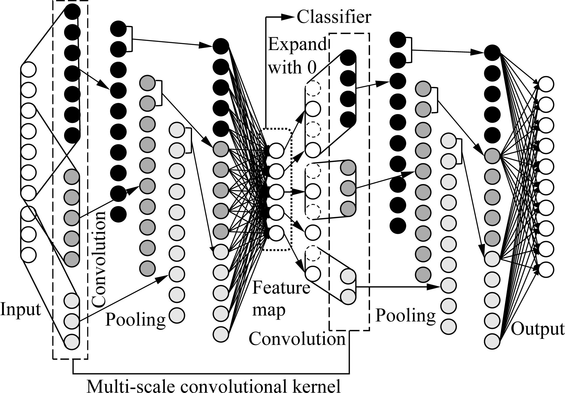
Fig.1 Structure of 1DMSCAE
The main advantage of a one-dimensional multi-scale convolutional auto-encoder is that it uses parallel convolutional kernels and deconvolutional kernels of different scales in the convolutional coding layer and deconvolutional decoding layer. Moreover, these multi-scale convolutional kernels are strong feature extraction tools, which can achieve a better recognition effect and higher generalization performance.
2.2 Construction of 1DMSCAE
The classifier of the 1DMSCAE model selects Softmax. In order to avoid over-fitting, the dropout technique is adopted in the full-connection layer of the training phase. The loss function optimization algorithm of the model uses the adaptive moments (Adam) algorithm[14]. In addition, the model adopts a one-dimensional convolutional and pooling structure to directly perform adaptive feature extraction and fault classification on the original time domain signal.
2.3 Process of concrete realization
As shown in Fig.2,the flowchart of the 1DMSCAE model can be divided into 4 steps:
1) Data set partitioning. The time domain acceleration signals of the bearings collected by the experiment are randomly divided into training sets and test sets according to a certain proportion.
2) Unsupervised training of the model. The back-propagation (BP) algorithm[15] is applied for the update of weights in the model. In the process of reconstructing the data by 1DMSCAE, the reconstruction error is back-propagated to achieve the effect of training feature extraction network.
3) Supervised training of the model. Perform back-propagation using the loss between the tagged data and the classifier output to fine tune the entire 1DMSCAE model parameters.
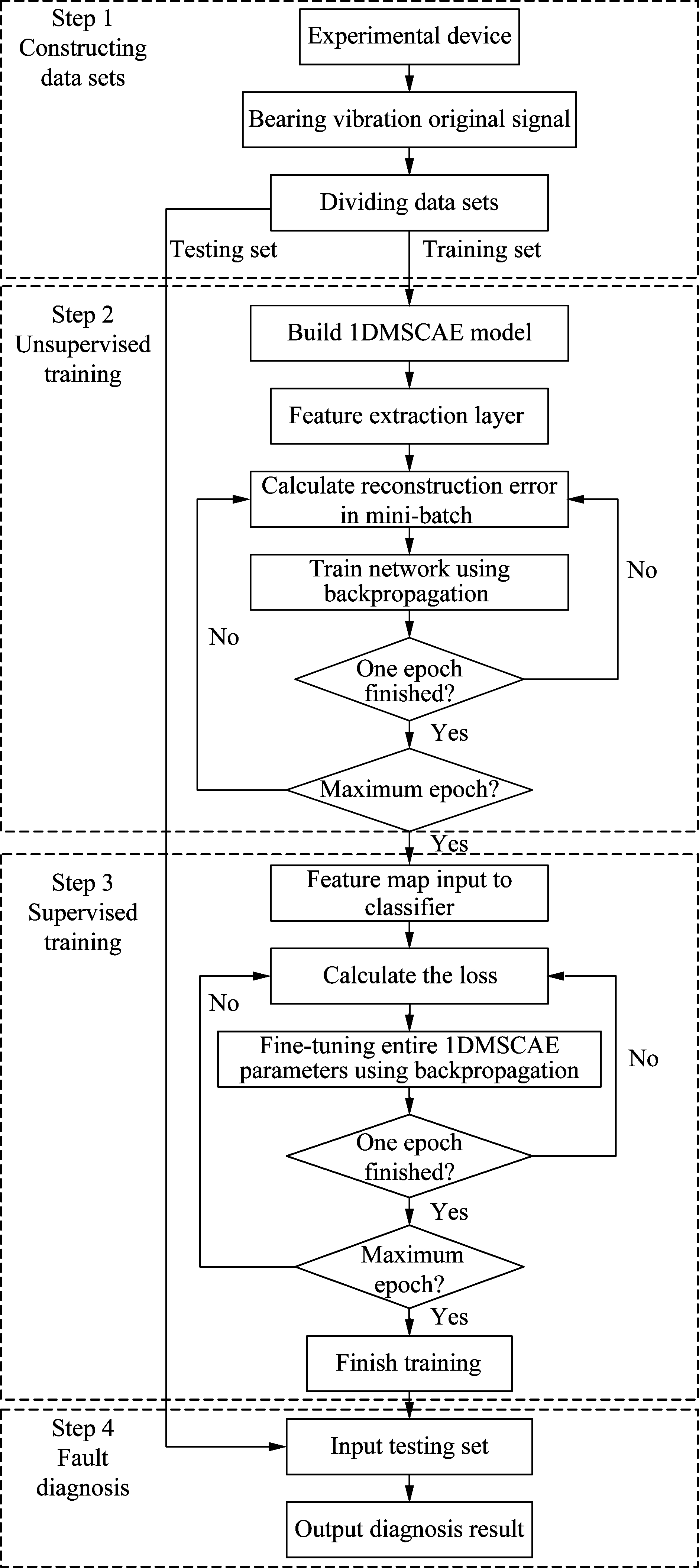
Fig.2 The flowchart of the proposed method
4) Testing of the model. Input the test data into the model, and the diagnosis results are obtained to verify the training effect of the model.
3 Experimental Verification
3.1 Simulation signal fault diagnosis and analysis
In order to verify the feasibility of the 1DMSCAE model in fault diagnosis, the 1DMSCAE model is applied to the simulation data set. The tool for signal simulation is Matlab 2016a.
3.1.1 Simulation signal description and analysis
This experiment constructs bearing outer and inner race faults by mimicking the failure mechanism.
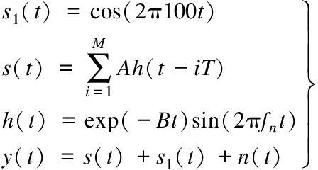
The simulation signal for the outer race fault is as follows:
(3)
where T=1/fo, fo is the characteristic frequency of the outer race fault, the size is 100 Hz; the system natural frequency fn=2 000; B is the resonance damping coefficient of the system and B=800 rad/s. The impact amplitude A is a constant, and n(t) is a Gaussian white noise with a signal-to-noise ratio of 0 dB.
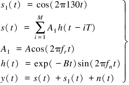
The simulation signal for the inner race fault is as follows:
(4)
where T=1/fi, fi is the characteristic frequency of the inner race fault, and the size is 130 Hz. A1 is an amplitude modulation signal; the period is 1/fr, and fr=50 Hz is the axis frequency. The resonance coefficient of the system is B=800 rad/s, and n(t) is Gaussian white noise with a signal-to-noise ratio of 0 dB.
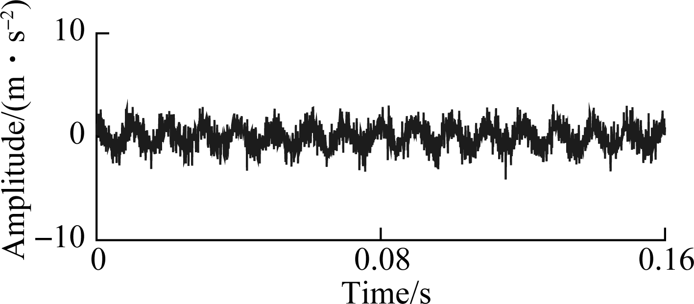
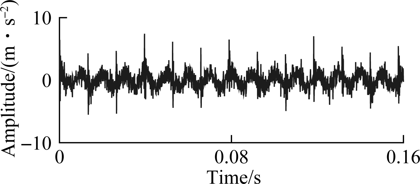
The sampling frequency is 12.8 kHz and the sampling time is 32 s. Constant A takes 1 and 6, which represents the signals of the two fault levels of the outer and inner race fault signals, respectively. This paper intercepts every 2 048 points as one sample, 200 samples per fault, and the time domain waveform of each sample is shown in Fig.3. Two-thirds of the samples are randomly selected as training signals, and the remaining one-third as test samples.
(a)

(b)
(c)

(d)
Fig.3 Fault simulation signal. (a) Outer race fault 1; (b) Outer race fault 2; (c) Inner race fault 1; (d) Inner race fault 2
3.1.2 Model parameter setting
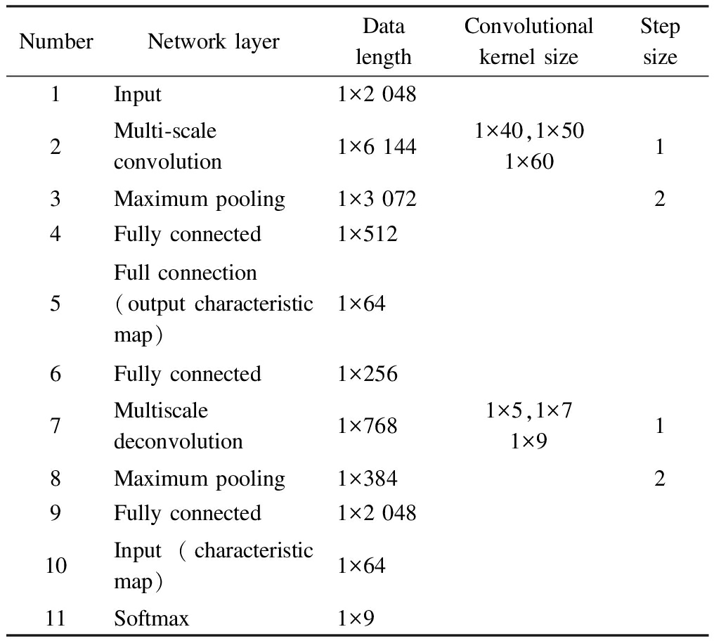
The parameter settings of the 1DMSCAE model are shown in Tab.1
Tab.1 1DMSCAE parameters settings
NumberNetwork layerData lengthConvolutional kernel sizeStep size1Input1×2 0482Multi-scale convolution1×6 1441×40,1×501×6013Maximum pooling1×3 07224Fully connected1×5125Full connection(output characteristic map)1×646Fully connected1×2567Multiscale deconvolution1×7681×5,1×71×918Maximum pooling1×38429Fully connected1×2 04810Input (characteristic map)1×6411Softmax1×9
3.1.3 Simulation signal reconstruction and diagnosis results
In order to analyze the signal reconstruction ability and feature extraction ability of the 1DMSCAE model, input a sample of the outer race fault 1 simulation signal (including 2 048 points) into the trained 1DMSCAE feature extraction network to obtain the original input and the reconstructed output. The comparison of the data curve is shown in Fig.4.
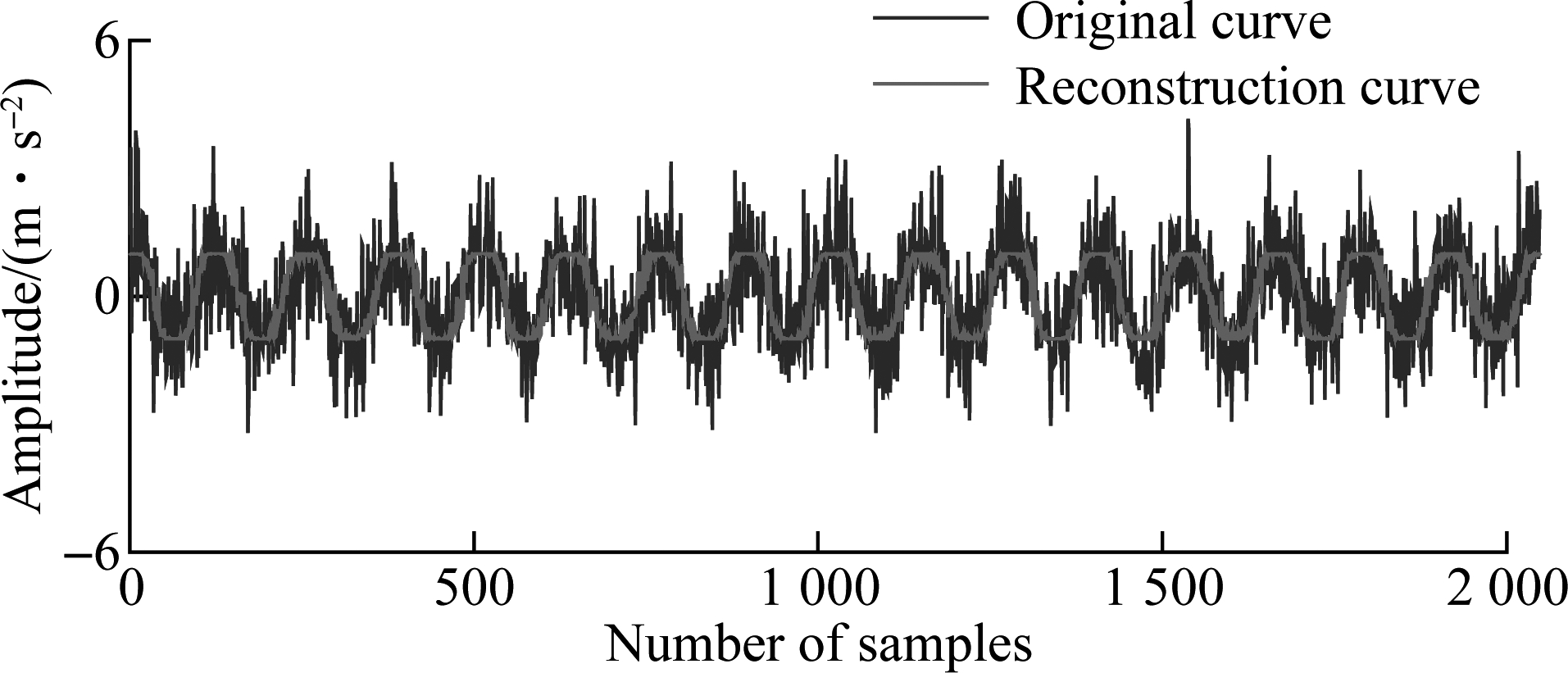
Fig.4 Comparison of reconstructed signal and original signal
It can be seen that the reconstructed data signal of the 1DMSCAE can restore the input signal while removing the influence of noise, and at the same time retain the characteristics of the signal well, so that the model has strong feature extraction ability.
In order to verify the superiority of the 1DMSCAE model feature extraction ability, this paper compares the feature classification performance with two common feature extraction methods and two normal deep learning models: principal component analysis (PCA) and non-negative matrix factorization (NMF), CNN, normal CAE, and then inputs the results of different feature extraction methods to softmax. In the experiment, five methods extract 64-dimensional features, and the results are shown in Tab.2.
Tab.2 Comparison of diagnostic results of features extracted by different methods

Method1DMSCAENormal CAECNNPCANMFAccuracy rate/%99.7593.2190.9481.2584.63
From Tab.2, we can see that the classification effect of 1DMSCAE on the extracted features is significantly better than those of the other four methods, and the classification accuracy rate is 99.75%, which is higher than 81.25% of the PCA method and 84.63% of the NMF method. The classification effect of 1DMSCAE is also better than those of normal CAE and CNN. It shows that 1DMSCAE has a stronger feature extraction ability, and that the extracted features can retain the original data information to a greater extent.
3.2 Bearing fault diagnosis experiment 1
Since the simulated signal cannot represent the bearing fault under real conditions, the open bearing data set of Case Western Reserve University is used for experimental analysis. The experimental apparatus includes an electric motor, a torque sensor, a power test meter, and an electronic controller. The data used in the experiment is acquired by an accelerometer placed above the bearing seat of the motor. The sampling frequency is 48 kHz and the load of the motor is 3 HP. The experimental system simulates three kinds of fault types of bearing: the outer race fault (OF), inner race fault (IF) and rolling ball fault (BF). Each fault type has three fault levels, including a damage diameter 0.007, 0.014, and 0.021 mm, so there are 9 fault states. Each of the fault states has 1 024 sample points, and each fault state has 200 samples.
3.2.1 Experimental conditions and network parameter selection
In hyperparameter selection, the size of the multi-scale convolutional kernel has a great influence on the feature extraction ability of the network. In order to select the convolutional kernel of the best scale, this paper selects a multiple of 10 single convolutional kernels for the recognition accuracy experiment. The experimental results are shown in Tab.3.
Tab.3 Test accuracy of different convolution kernel sizes
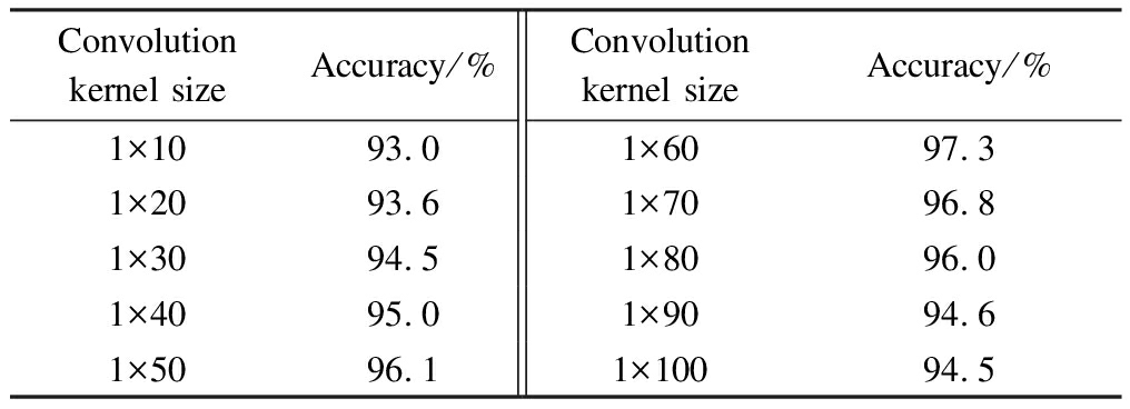
Convolution kernel sizeAccuracy/%Convolution kernel sizeAccuracy/%1×1093.01×6097.31×2093.61×7096.81×3094.51×8096.01×4095.01×9094.61×5096.11×10094.5
Considering that the convolutional kernel has a fitting phenomenon when the size is too large, too many kernels will affect the computational efficiency of the model. The model selects three convolutional kernels, and the sizes of the convolutional kernels are 1×30,1×50, 1×70, respectively. The dropout rate is 0.2.
In order to compare the effect of the activation function on the recognition accuracy, this paper compares three common activation functions, and the results are shown in Tab.4.
Tab.4 Test accuracy of different activation function%

Convolutional layerFully connected layerReluSigmoidTanhRelu83.15±2.677.47±3.469.92±7.1Sigmoid95.87±1.879.48±4.171.84±5.8Tanh99.21±0.0973.09±3.667.22±6.6
Therefore, the activation function of convolutional layer is relu, and the activation function of the fully connected layer is tanh.
In this experiment, the learning rate of the feature extraction network is 0.000 1, the learning rate of the classifier is 0.000 2, and the training iterations number of feature extraction layer is 150. The iterations number of the classifier is 70. The hardware environment in which the model runs is Intel i5-7300HQ+Nvidia 1050, and the software environment is Python+ Tensorflow.
3.2.2 Experimental results and analysis
In order to verify the recognition performance of the proposed model and the current common fault diagnosis algorithm, the comparison methods are BP-NN, SVM, one-dimensional convolutional neural network (CNN) and normal one-dimensional convolutional auto-encoder (CAE). CNN and CAE comprise of two layers of the convolutional layer, two layers of the pooling layer and two layers of the full-connected layer. The convolutional kernels are 1×50 and 1×30, respectively. When the data length in the deconvolution process is insufficient and needs to be filled, the all-zero padding is used. The Gaussian kernel function is chosen for SVM because there are fewer features and the size of the sample is medium. The kernel parameter and penalty factor of SVM are 30 and 0.1, respectively. The input layer of the BP neural network, the number of hidden layer and output layer units are 500, 200 and 9, respectively, and the activation function is sigmoid. The learning rate is 0.1 and the iteration number is 500. The results of the diagnosis are shown in Fig.5.
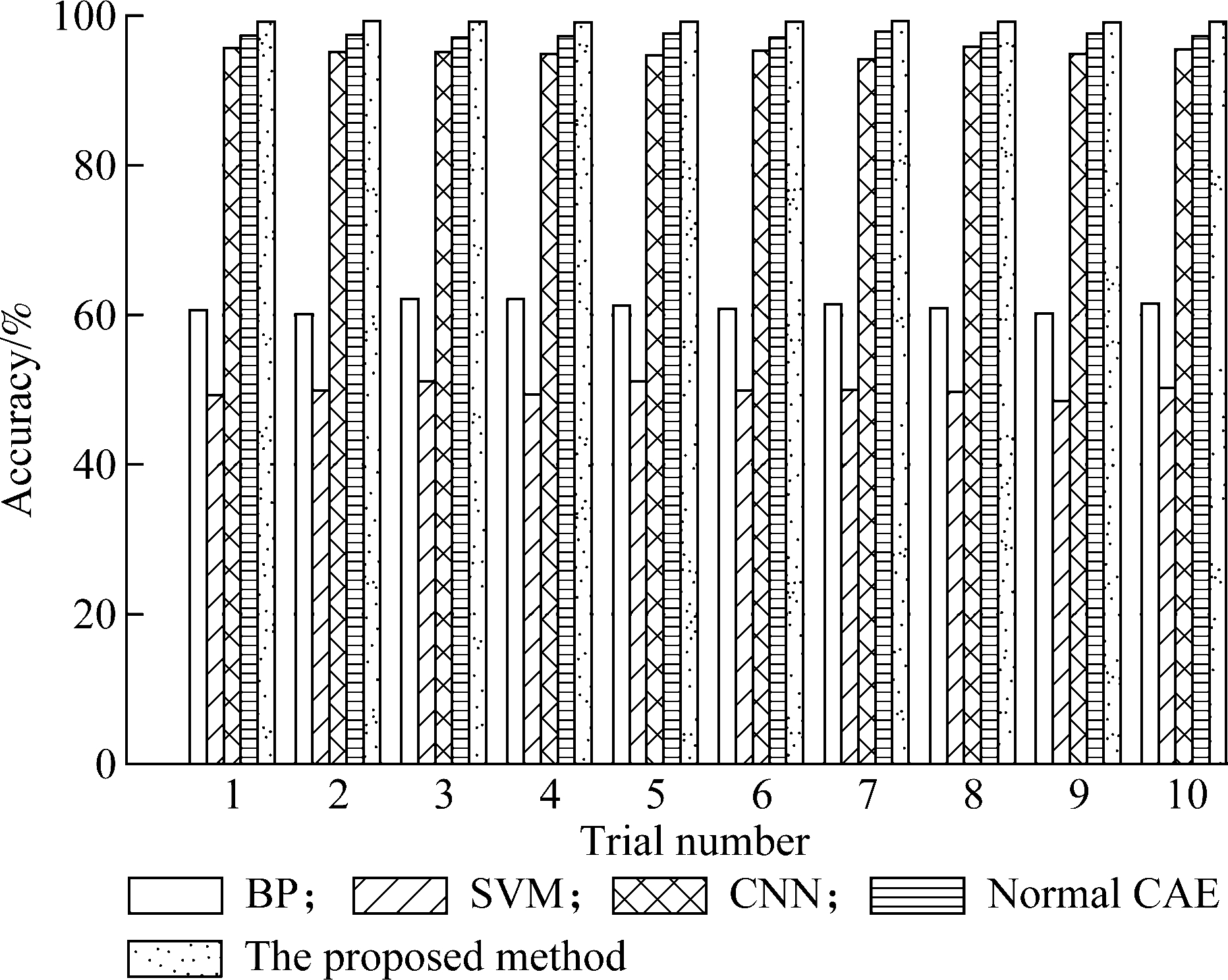
Fig.5 Results of the bearing fault diagnosis using different methods
From the comparison results of the six models, we can see that the proposed model has a higher diagnostic accuracy than the traditional machine learning network. The reason is that the shallow network of traditional machine learning has a weak feature extraction capability and cannot classify faults effectively[16]. Compared with the CNN and CAE models, the diagnostic accuracy of the 1DMSCAE model is also improved. This is because the CNN network lacks the process of unsupervised training to extract data features, which makes the network unable to achieve higher precision since it may fall into the local optimum. Compared with the common CAE model, 1DMSCAE with a multi-scale convolutional kernel can achieve better diagnostic accuracy due to its stronger feature extraction ability.
3.3 Bearing fault diagnosis experiment 2
To further verify the performance of the proposed model, the CAE and 1DMSCAE models were further compared on the laboratory dataset. The bearing test system used in the laboratory consists of the experimental head, transmission system, loading system, electrical control system, test and data acquisition system. As shown in Fig.6(a), four 6205 rolling bearings with different faults are installed at the same time, and four acceleration sensors are used to collect vibration signals on four rolling bearing rigid shells. The four fault types are rolling ball fault, outer race fault, inner race fault and composite fault of inner race and outer race. The bearing load during the experiment is 0, the bearing speed is 1 050 r/min, and the sampling frequency is 10 240 Hz. The experimental sample length is 2 048 points, and each fault state has 200 samples, for a total of 800 samples.
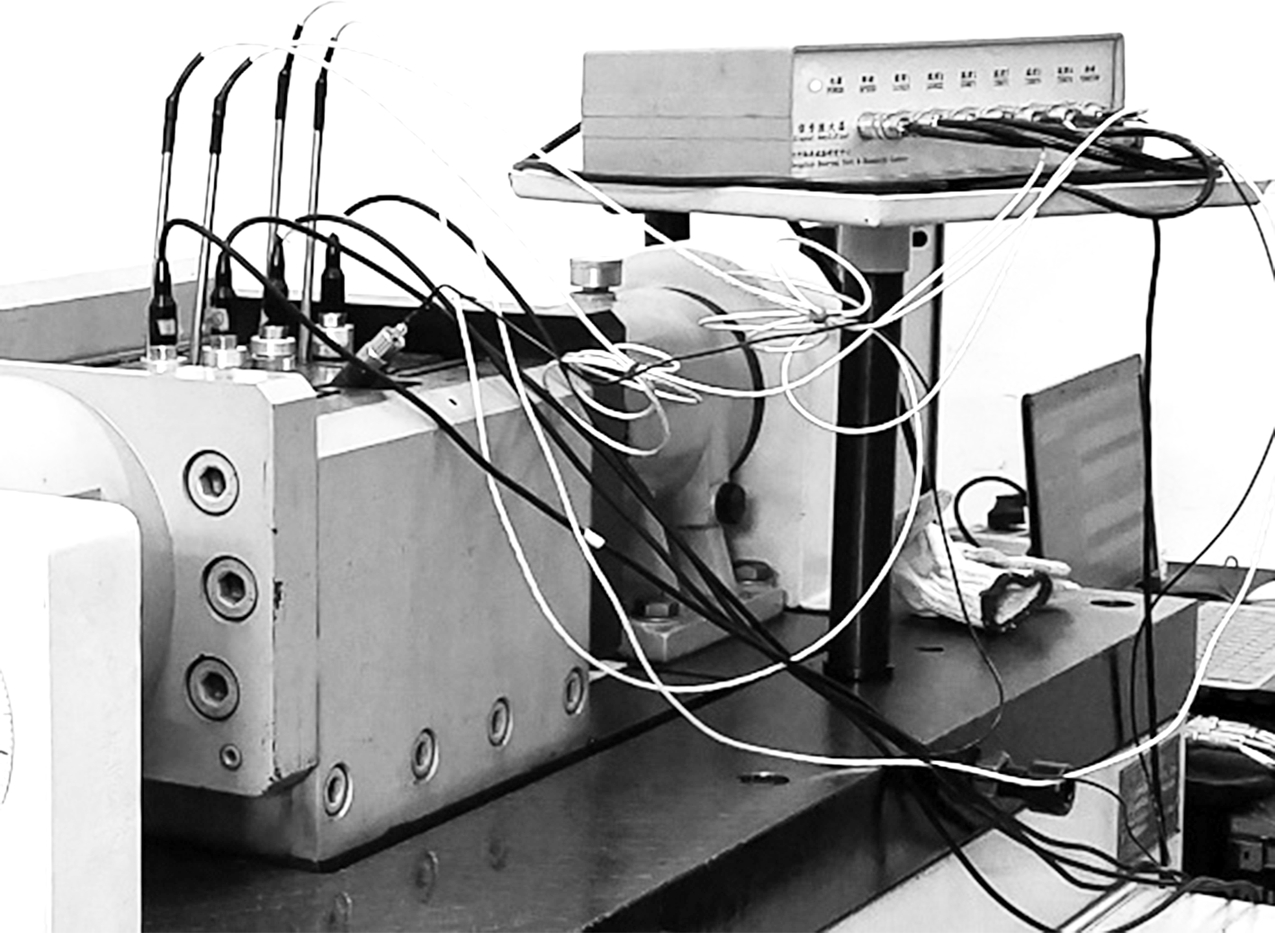
(a)
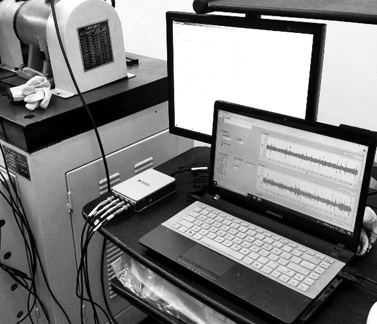
(b)
Fig.6 Equipment of the experiment. (a) Sensor installation;
(b) Data acquisition
In the experiment, the CAE and 1DMSCAE network parameters only adjust the input and output data lengths to 2 048 and the learning rate to 0.001 compared to the network verified by the Western Reserve University data. The experiment records the average value of every 10 experiments, and records them ten times.
Fig.7 shows that in the case of fewer fault types, the model proposed in this paper has an excellent diagnostic capability, and that the accuracy of the method is stable at 100%, while the accuracy of normal CAE is between 99.95% and 99.99%. This shows that the one-dimensional multi-scale convolutional auto-encoder has a stronger feature extraction capability than the normal convolutional auto-encoder.
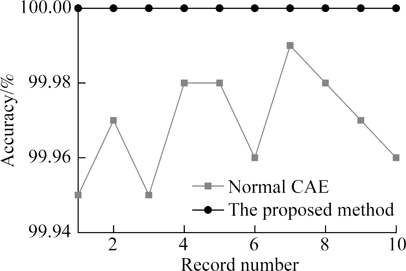
Fig.7 Comparison of accuracy
The loss of the reconstructed signal on the original signal reflects the ability of the model to restore the input signal, and also reflects its ability to extract the features from the input data. In order to compare the reconstruction ability of the model to the original input signal, the 1DMSCAE model is compared with the normal CAE in signal reconstruction error. The reconstruction error uses the root mean square error (RMSE).
As shown in Fig.8, as the training progresses, the reconstruction error of the proposed method can be reduced more quickly and achieve a lower effect. When the epoch exceeds 80, the reconstruction errors of normal CAE and 1DMSCAE are stable at 0.092 5 and 0.090 5, respectively. Therefore, the 1DMSCAE model can better restore the data after the dimensionality reduction of the signal, which means that the extracted feature map of 1DMSCAE can better represent the original signal than normal CAE.
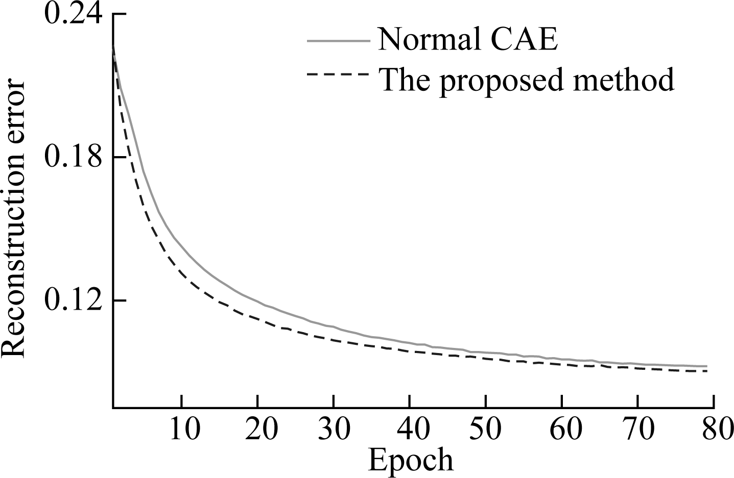
Fig.8 Comparison of the reconstruction error
4 Conclusions
1) The proposed model can effectively realize the automatic feature extraction and fault diagnosis of fault data, and can avoid the dependence of traditional methods on expert experience and signal processing knowledge.
2) The one-dimensional multi-scale convolutional auto-encoder can effectively extract the features of the data during the process of reconstructing the input data.
3) Compared with a single convolutional kernel, the multi-scale convolutional kernel and deconvolutional kernel of the network can achieve better diagnostic results.
4) The 1DMSCAE model proposed in this paper has many convolutional kernels. The size and number of multi-scale convolutional kernel and deconvolutional kernel need to be adjusted step by step in a large number of experiments to achieve better performance. The next step is to study the adaptive convolutional kernel parameter selection model to further improve the generalization ability of the model.
[1]Li H, Xiao D Y. Survey on data driven fault diagnosis methods[J]. Control and Decision, 2011, 26(1): 1-9, 16. DOI:10.13195/j.cd.2011.01.3.lih.016.(in Chinese)
[2]Ren H, Qu J F, Chai Y. Research status and challenges of deep learning in fault diagnosis[J]. Control and Decision, 2017, 32(8):1345-1358. (in Chinese)
[3]Hinton G E. Reducing the dimensionality of data with neural networks[J]. Science, 2006, 313(5786): 504-507. DOI:10.1126/science.1127647.
[4]Lei Y G, Jia F, Zhou X. Mechanical equipment big data health monitoring method based on deep learning theory[J]. Journal of Mechanical Engineering, 2015, 51(21):49-56. (in Chinese)
[5]She D M, Jia M P. Wear indicator construction of rolling bearings based on multi-channel deep convolutional neural network with exponentially decaying learning rate[J]. Measurement, 2019, 135: 368-375. DOI:10.1016/j.measurement.2018.11.040.
[6]Zhao R, Yan R Q, Chen Z H, et al. Deep learning and its applications to machine health monitoring[J]. Mechanical Systems and Signal Processing, 2019, 115: 213-237. DOI:10.1016/j.ymssp.2018.05.050.
[7]LeCun Y, Bottou L, Bengio Y, et al. Gradient-based learning applied to document recognition[J]. Proceedings of the IEEE, 1998, 86(11): 2278-2324. DOI:10.1109/5.726791.
[8]Liu X C, Zhou Q C, Zhao J, et al. Real-time anti-noise fault diagnosis algorithm for one-dimensional convolutional neural networks[J]. Journal of Harbin Institute of Technology, 2019, 51(7):89-95.(in Chinese)
[9]Zhang W, Peng G L, Li C H. Bearings fault diagnosis based on convolutional neural networks with 2-D representation of vibration signals as input[J]. MATEC Web of Conferences, 2017, 95: 13001. DOI:10.1051/matecconf/20179513001.
[10]Masci J, Meier U, Cire an D, et al. Stacked convolutional auto-encoders for hierarchical feature extraction[M]//Lecture Notes in Computer Science. Berlin, Heidelberg: Springer Berlin Heidelberg, 2011: 52-59. DOI:10.1007/978-3-642-21735-7_7.
[11]Li F F, Qiao H, Zhang B. Discriminatively boosted image clustering with fully convolutional auto-encoders[J]. Pattern Recognition, 2018, 83: 161-173. DOI:10.1016/j.patcog.2018.05.019.
[12]Liu X C, Zhou Q C, Zhao J, et al. Fault diagnosis of rotating machinery under noisy environment conditions based on a 1-D convolutional autoencoder and 1-D convolutional neural network[J]. Sensors, 2019, 19(4): 972-993. DOI:10.3390/s19040972.
[13]Zhang X N, Xiang Z, Tang C H. A deep convolutional autoencoder and its application in fault diagnosis of rolling bearings[J]. Journal of Xi’an Jiaotong University, 2018, 52(7):6-13,64. (in Chinese)
[14]Kingma D P, Ba J. Adam: A method for stochastic optimization[J/OL].Computer Science, 2014. https://arxiv.org/pdf/1412.6980v8.pdf.
[15]Rumelhart D E, Hinton G E, Williams R J. Learning representations by back-propagating errors[J]. Nature, 1986, 323(6088): 533-536. DOI:10.1038/323533a0.
[16]Lei Y G, Jia F, Lin J, et al. An intelligent fault diagnosis method using unsupervised feature learning towards mechanical big data[J]. IEEE Transactions on Industrial Electronics, 2016, 63(5): 3137-3147. DOI:10.1109/tie.2016.2519325.