High frequency of wet weather accidents is partly caused by hydroplaning and reduced skid resistance of asphalt pavement[1]. The thickness of the water film caused by rainfall is one of the factors contributing to the reduction of skid resistance on wet pavements[2], which is closely related to rainfall intensity, slope gradient, and slope length[3]. Numerous experimental studies have indicated that the pavement skid resistance decreases with the increase in the water film thickness (WFT), and the skid resistance performance of new pavements is better than that of old pavements under the same WFT[4-5]. However, it is generally a challenge to measure the WFT directly on the pavements. Additionally, pavement transverse and longitudinal slopes are not considered in most of the existing models/formulae, which often leads to inaccurate computations and results. Therefore, it is prudent to formulate more representative and realistic models for characterizing/quantifying the WFT and recommend appropriate skid-resistance performance indices for wet pavements; thereby, contributing to the optimization of driving safety conditions in adverse weather.
Based on the above background, this paper formulated and preliminarily validated a mathematical model for characterizing and quantifying the WFT and skid-resistance, which also takes the pavement longitudinal and transverse slopes into account. Using the British pendulum experimental data, the skid-resistance, quantified in terms of the British pendulum number (BPN), was measured and modeled under different rainfall intensities, pavement transverse and longitudinal slopes. Modifications and revisions which are related to the BPN and sideway force coefficient (SFC60) with respect to new asphalt pavements, and the stopping sight distance (SSD) with respect to rainfall intensities and longitudinal slopes, are also proposed in the paper. Finally, safe driving speeds are determined using the safety driving model proposed in this paper along with some recommendations for speed limit strategies under wet weather.
1 Water Film Thickness Model
1.1 Theoretical formulation of the WFT model
There are laminar flow and turbulent flow in fluid motions, which can be classified by the Reynolds number. The slope flow on pavement surfaces is turbulent flow[6], which can be simplified to uniform flow in a rectangular open channel. The Reynolds number of open channel flow is expressed as
(1)
where nRe is the Reynolds number; v is the average velocity, m/s; R is the hydraulic radius, m, R=A/χ, where A is the cross-sectional area of the channel and χ is the wetted perimeter of the channel; υ is the kinematic viscosity of water; and the default value is 1×10⁻⁶m2/s.
The cross-sectional area is computed as A=bh with a given water film width b and water film thickness h. The wetted perimeter is computed as χ=b+2h. Thus, Eq.(1) can be reduced to
(2)
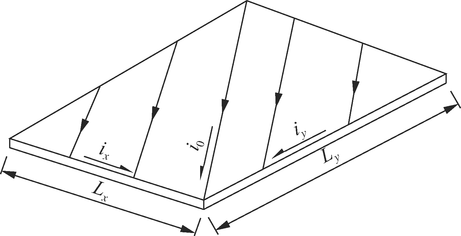
Fig.1 shows the schematic diagram of slope flow on a pavement surface, where ix is the transverse slope gradient; iy is the longitudinal slope gradient; i0 is the resultant slope gradient; Lx is the horizontal length of the slope, m; Ly is the longitudinal length of the slope, m.
(a)

(b)
Fig.1 The slope flow on a pavement surface. (a) Direction of the slope flow; (b) Profile of the slope flow
According to the design specification for highway alignment (JTG D20—2017)[7], the resultant slope gradient of the highway pavement is supposed to be less than 10.5%. So, the projection length of the pavement surface on the horizontal plane is approximately equal to its actual slope length, and the water depth in the vertical direction is approximately equal to its direction perpendicular to the slope surface.
The unit-width discharge q(m2/s) is defined as the product of the average velocity and the water film thickness. Thus, the Reynolds equation can be represented as
(3)
From the momentum equation of slope flow[4], the hydraulic gradient J is equal to the resultant slope i0, which is shown as follows:
(4)
where L is the slope length, m; hf is the frictional head loss, m.
The friction head loss is given by Darcy-Weisbach’s formulation as[6]
(5)
where λ is the friction factor; R is the hydraulic radius, R=h; g is the acceleration due to gravity, generally g=9.81 m/s2.
The friction factor is obtained from Eqs.(4) and (5),
(6)
For turbulent flow, the friction factor λ can be calculated using Blasius equation[8]:
(7)
Considering Eqs.(3), (6) and (7), the following equation is proposed:
(8)
The equation for total discharge computation is adopted from the specifications for the drainage design of highway (JTG/T D33-2012)[9] as
Q=16.67ψIF
(9)
where Q is the total discharge, m3/s; ψ is the runoff coefficient, generally ψ=0.95 for asphalt pavements; I is the rainfall intensity, mm/min, ranging from 0.5 to 3 mm/min; F is the catchment area, km2.
The catchment width is assumed to be unit width, that is Q=q. The WFT equation based on resultant slope gradient can be derived from Eq.(8) and Eq.(9) as
(10)
1.2 Verification of the theoretical formula
The reliability of the proposed theoretical formulation was verified by comparing the theoretical formulation with the empirical formulae recommended by British scholars and the experimental regression model proposed by He[4]. The WFT model was calculated with a rainfall intensity of 2 mm/min, and a resultant slope of 2% with the unit-width catchment area was converted into slope length, F=1×10⁻⁶L. The graphical results are shown in Fig.2.
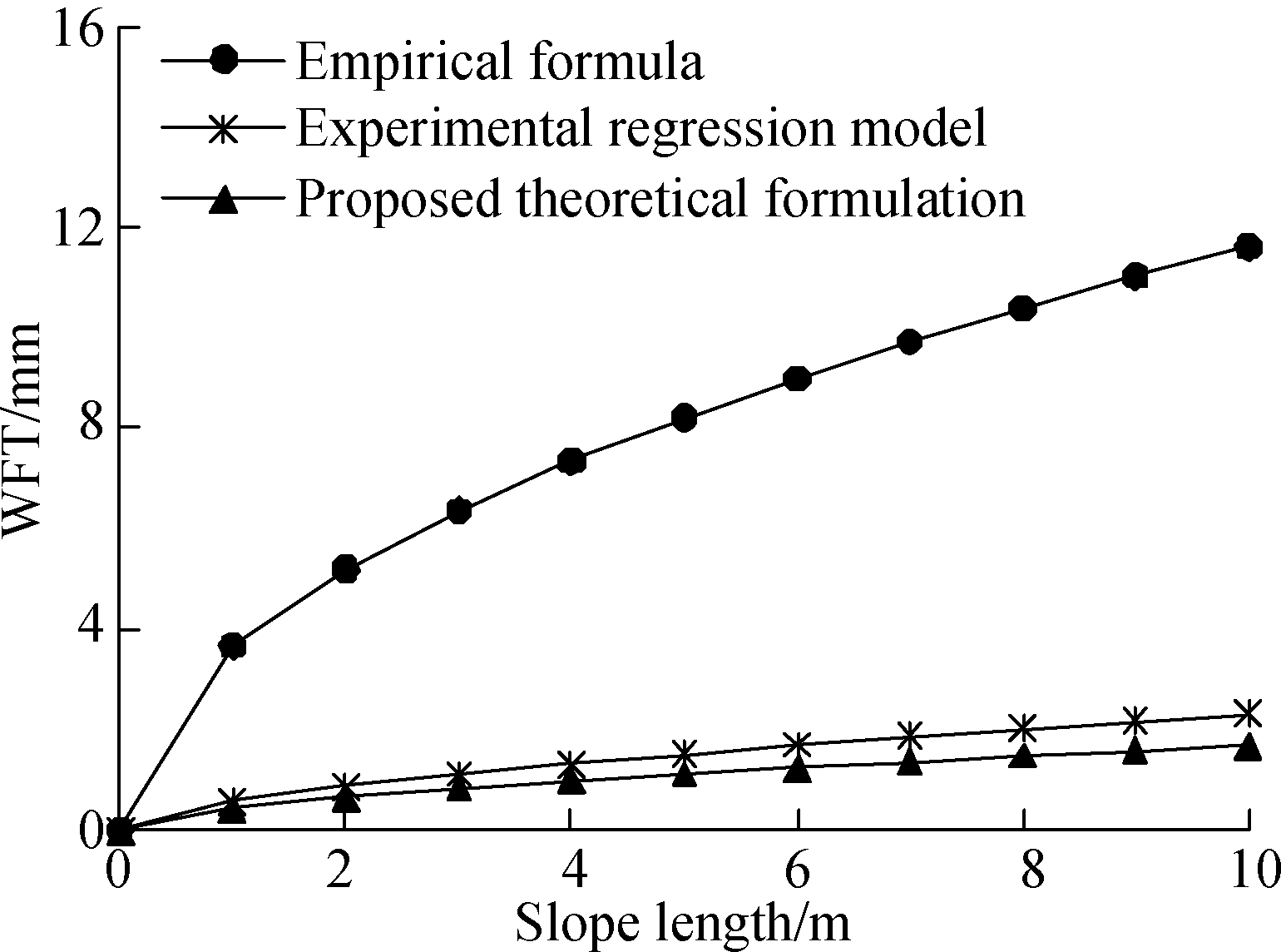
Fig.2 Comparison of WFT formulae
Fig.2 shows that the theoretical formula has a good correlation with the experimental regression model proposed by He[4], which is characterized by a nonlinear increasing trend with the increase in slope length. Compared to the low accuracy of empirical formula, highly targeted experimental regression models, based on Fig.2, appear to be more suitable for asphalt pavements, which indicates that the theoretical formulation in this paper is reasonable and practical.
1.3 Slope-based WFT model formulation
In this paper, it is assumed that the driving direction is longitudinal and the direction perpendicular to the driving direction is transverse. So, the resultant slope of the pavement i0 is
(11)
As shown in Fig.1, the unit-width catchment area F is expressed as
(12)
where Fx is the projection area of the unit-width catchment area on the cross section, which is the same as the unit-width area from the road edge to the road centerline, km2.
According to Eqs.(10) to (12), the model for computing the WFT, based on longitudinal and transverse slopes, can be formulated as
(13)
2 WFT Effects on Pavement Skid Resistance
2.1 BPN variation with WFT
Based on different WFT levels, Zhao et al.[10] and He[4] measured the BPN on asphalt pavements with a texture depth of 1.02 and 1.40 mm for new SMA-13 pavements, 0.43 mm for old SMA-13 pavements, 0.92 mm for new AC-13 pavements, and 0.62 mm for old AC-13 pavements. The new pavement was represented by a specimen made in the laboratory and the old pavement had a service life of 5 years. The test results are listed in Tab.1.
Tab.1 BPN of different pavements under different WFT levels
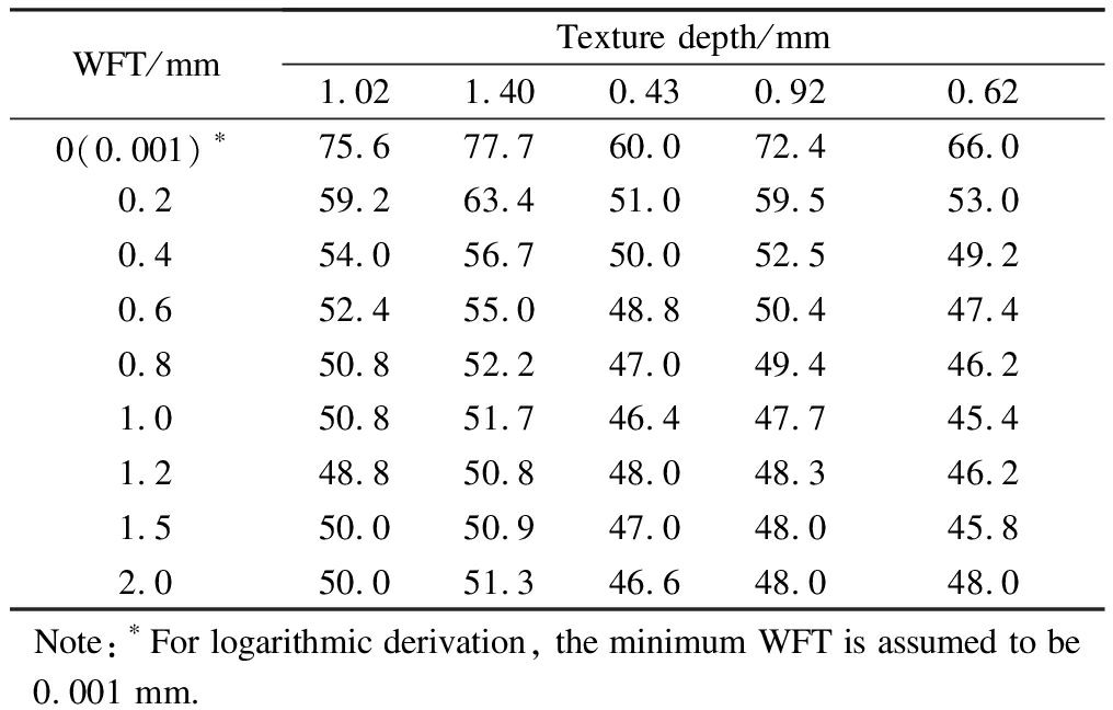
WFT/mmTexture depth/mm1.021.400.430.920.620(0.001)∗75.677.760.072.466.00.259.263.451.059.553.00.454.056.750.052.549.20.652.455.048.850.447.40.850.852.247.049.446.21.050.851.746.447.745.41.248.850.848.048.346.21.550.050.947.048.045.82.050.051.346.648.048.0Note:∗For logarithmic derivation, the minimum WFT is assumed to be 0.001 mm.
When the WFT is greater than 2 mm, the BPN values rebound, which indicates that water comes into contact with the pendulum edge as well as the rubber slider, resulting in larger BPN values. Therefore, the WFT greater than 2 mm is excluded from Tab.1.
Veith[11] found a logarithmic relationship between BPN and WFT. Taking the new SMA-13 pavement with a texture depth of 1.02 mm as an example, the logarithmic regression curve of BPN vs. WFT is shown in Fig.3.
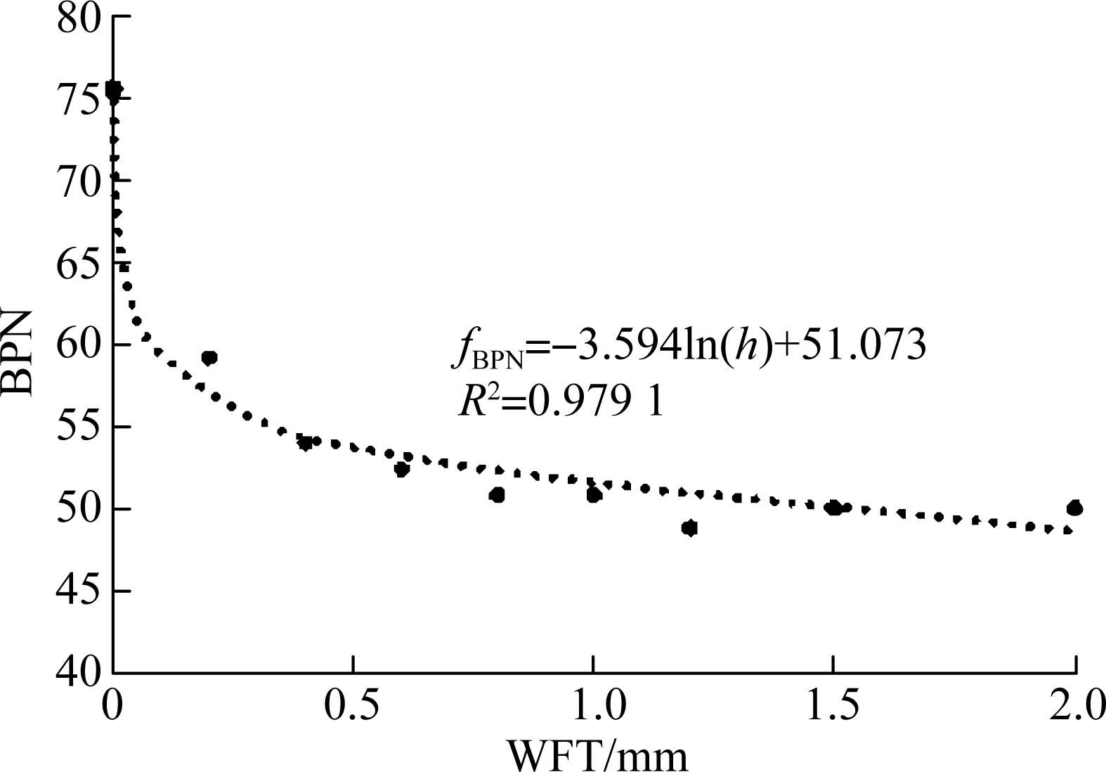
Fig.3 Logarithmic regression curve of BPN vs. WFT for new SMA-13 pavement
Fig.3 shows that the BPN decreases with the increase in the WFT, which indicates a reduction in the pavement skid resistance. However, the BPN decreases rapidly within 0.5 mm when the thin layer of water covering the pavement surface acts like a lubricant and reduces the contact between the tires and the pavement surface. Also, there is an inflection point at about 0.5 mm, after which the slope, i.e., the rate of decline, changes significantly, tending towards stability. In this situation, the water film covers the micro-textures of the pavement surface, and reduces the adhesion component of the friction.
The regression equation of BPN vs. WFT for the asphalt pavement is given as
fBPN=aln(h)+b
(14)
where fBPN is the value of BPN; h is the value of WFT; a and b are the regression coefficients.
The BPN regression coefficients, a, b, and R2 values for different pavement texture depths are shown in Tab.2.
Tab.2 BPN regression coefficients for different pavement texture depths

RegressioncoefficientsTexture depth/mm0.430.620.901.021.40a-1.810-2.744-3.437-3.594-3.730b47.63546.97949.51851.07352.950R20.973 10.951 40.950 70.979 10.955 1
The regression coefficients a and b are well correlated with the texture depth as shown below:
(15)![]()
(16)
where dTD is the texture depth of the asphalt pavement, mm.
2.2 BPN vs. rainfall intensity and slopes
Combining Eq.(13) with Eq.(14), the function of BPN is obtained as
(17)
Relating the BPN equation of different asphalt pavements to rainfall intensity, longitudinal and transverse slopes, a simplified form of Eq.(17) is obtained after substituting the known variables.
(18)
2.3 Skid resistance-rainfall intensity and slopes
The impacts of rainfall intensity and pavement geometry on pavement skid resistance are expressed in Eqs.(17) and (18).
2.3.1 Impact of rainfall intensity
Fx is the unit-width area of one lane, namely Fx=3.75m2 = 3.75×10⁻⁶km2. The longitudinal and transverse slopes are both taken to be 2%. From the specifications for drainage design of highway (JTG/T D33—2012)[9], the design recurrence interval of rainfall for surface drainage of the expressway and first-class highway pavements and shoulder is 5 years. In the calculation process, the rainfall intensity varies from 0.20 to 3.00 mm/min, taking the texture depth of 0.5, 1.0 and 1.5 mm, respectively. The graph results are shown in Fig.4.
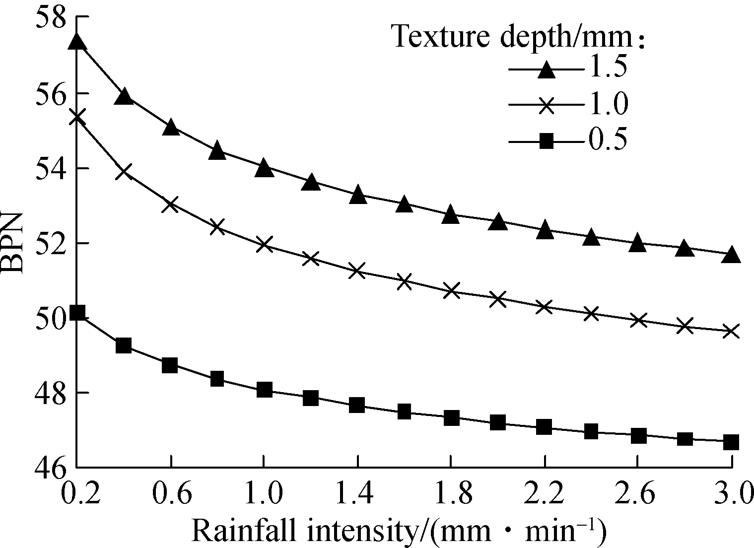
Fig.4 Variation of BPN with the change of rainfall intensity
Fig.4 indicates that rainfall intensity is a key contributor to the decline of wet-pavement skid resistance.BPN values decreases exponentially as the rainfall intensity increases. The rate at which BPN values decrease generally becomes smaller as the rainfall intensity increases. Thereafter, the BPN values decrease at a much slower rate, which means that the rate of decay in the pavement skid resistance decreases slightly with the increase in WFT. However, sufficient texture depth helps to improve pavement skid resistance.
2.3.2 Impact of transverse slopes
Likewise, the outcomes for BPN under different transverse slopes are presented in Fig.5 by substituting a rainfall intensity of 2 mm/min, Fx of 3.75×10⁻⁶km2 and longitudinal slope of 2% into Eq.(17) or Eq.(18). As shown in Fig.5, BPN increases gradually with the increase in the transverse slope. Therefore, increasing the transverse gradients appropriately based on the need for drainage will likely improve the pavement skid resistance under wet weather conditions.
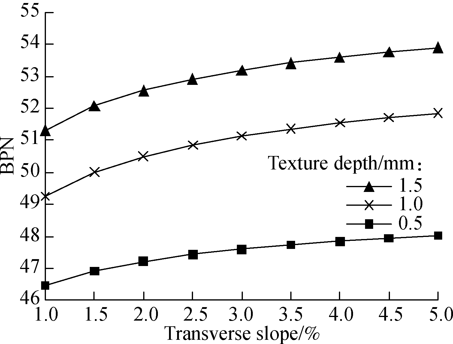
Fig.5 Variation of BPN with the change of transverse slopes
2.3.3 Impact of longitudinal slopes
Similarly,the results of BPN under different longitudinal slopes are shown in Fig.6 by substituting a rainfall intensity of 2 mm/min, Fx of 3.75×10⁻⁶km2 and transverse slope of 2% into Eq.(17) or Eq.(18). From Fig.6, it is clear that the BPN value decreases slowly with the increase in the longitudinal slope gradient, which is opposite to the trend exhibited by the transverse slope. This means that the effect of the longitudinal slope on the BPN value is not as critical as that of transverse slope. Therefore, skid resistance improvements should focus on the transverse and not on longitudinal slopes.
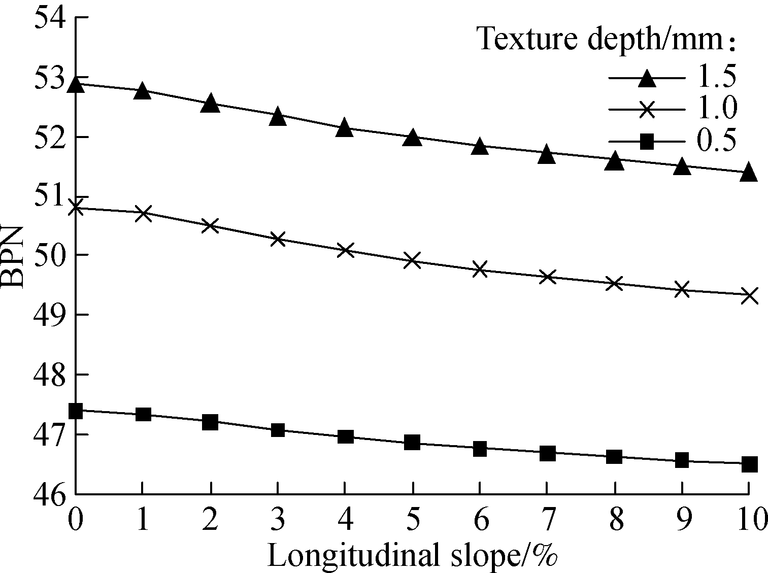
Fig.6 Variation of BPN with the change of longitudinal slopes
2.4 BPN-SFC60 correlations and rainfall intensity
Current specifications on the measurement of BPN, a friction index used to evaluate the skid resistance performance of asphalt pavements, is merely based on a moist pavement, and the impact of WFT under different rainfall intensities is not taken into account. Also, SFC60 is classified according to the mean annual precipitation, which does not correspond to or represent the most unfavorable state of a pavement. Therefore, the proposed values for BPN and SFC60 testing requirements for newly built asphalt pavements in different regions were proposed herein using the rainfall intensities as the classification criteria.
According to the 10-min rainfall intensity contour map of China with a recurrence period of 5 years, the designed rainfall intensities are divided into six categories: 0.5, 1.0, 1.5, 2.0, 2.5 and 3.0 mm/min[9]. These values are adopted in this paper.
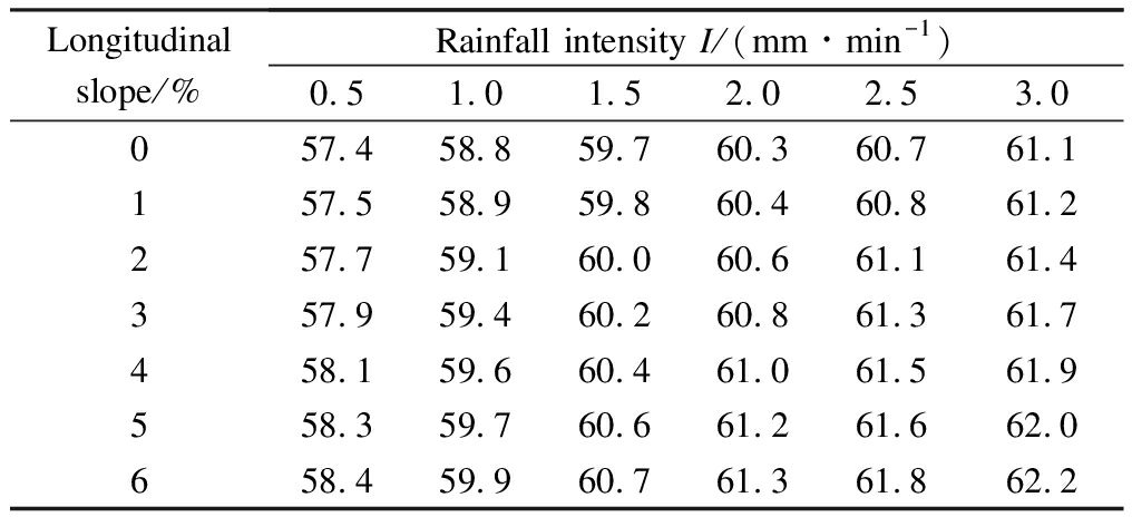
Based on Eqs.(13) and (18), taking transverse slope of 2%, Fx of 3.75×10⁻⁶ km2, the texture depth of 1.0 mm, and a longitudinal slope from 0% to 6%, the BPN testing requirements for new asphalt pavements under different rainfall intensities can be obtained as shown in Tab.3.
Tab.3 BPN testing requirements
Longitudinalslope/%Rainfall intensity I/(mm∙min-1)0.51.01.52.02.53.0057.458.859.760.360.761.1157.558.959.860.460.861.2257.759.160.060.661.161.4357.959.460.260.861.361.7458.159.660.461.061.561.9558.359.760.661.261.662.0658.459.960.761.361.862.2
Similarly, according to the conversion formula Eq.(19) of BPN and SFC60 from Chinese specifications for the design of highway asphalt pavement (JTG D50—2006)[12], the SFC60 testing requirements for new asphalt pavements under different rainfall intensities are obtained as shown in Tab.4.
fBPN=0.406 4fSFC+36.353
(19)
where fSFC is the value of SFC60.
Tab.4 SFC60 testing requirements
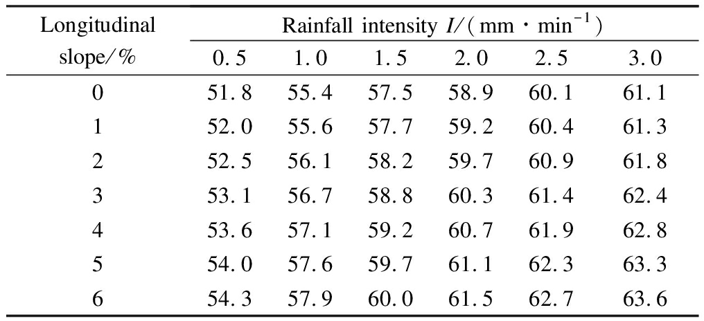
Longitudinal slope/%Rainfall intensity I/(mm∙min-1)0.51.01.52.02.53.0051.855.457.558.960.161.1152.055.657.759.260.461.3252.556.158.259.760.961.8353.156.758.860.361.462.4453.657.159.260.761.962.8554.057.659.761.162.363.3654.357.960.061.562.763.6
For the BPN testing requirements for new asphalt pavements in Tab.3 and taking the design rainfall intensity of 2 mm/min with a longitudinal slope of 2% as an example, the BPN value measured by T 0964—2008 during the acceptance inspection should meet fBPN≥60.6. Similarly, for SFC60 testing requirements for new asphalt pavements from Tab.4, the SFC60 value measured by T0965—2008 or T0967—2008 should meet the SFC60≥59.7 acceptance criteria.
Compared with the BPN requirements and the SFC60 requirements stipulated in Clause 7.1.2 of the Chinese specifications for design of highway asphalt pavement (JTG D50—2006)[12], the testing requirements proposed in this paper consider the rainfall intensity of each region, instead of the annual rainfall averages, which is more accurate. Thus, these test propositions, which are more representative, offer a promising reference value for the skid resistance performance testing of new asphalt pavements.
3 Wet-Weather Driving Safety Analysis
3.1 Wet-weather SSD model
Stopping sight distance (SSD) is the minimum sight distance available on a highway at any spot having sufficient length to enable the driver to stop a vehicle traveling at the design speed, safely without collision with any other obstruction. Conceptually, the SSD is the sum of the brake reaction distance and the braking distance. These two components can be mathematically expressed as[13]
(20)
where ST is the value of SSD, m; V is the operating speed, km/h; t is the driver perception-reaction time, 2.5 s; φ is the friction coefficient between the tires and the pavement surface, φ=BPN/100; ψ is the road resistance coefficient, ψ=fr+iy, where fr is the rolling resistance coefficient, and iy is the percent grade.
The operating speed is usually taken as 85% of the design speed when the design speed is 80 to 120 km/h and 90% of the design speed when the design speed is 40 to 60 km/h[7].
Zheng et al.[14] found that the friction coefficient between tires and the pavement surface is inversely proportional to the vehicle speed, and the regression formula of the friction coefficient and the vehicle speed is given as
φ2=φ1+0.002 5(V1-V2)
(21)
where φ1 is the friction coefficient when the vehicle speed is V1; φ2 is the friction coefficient when the vehicle speed is V2.
Yin et al.[15] found that when the vehicle speed is greater than 50 km/h, the rolling resistance coefficient can be calculated according to the following equation:
fr=0.011 6+0.000 142V
(22)
Combining Eqs.(20), (21) and (22), the SSD formula represented by BPN is obtained as
(23)
Based on the BPN formulation deduced in this paper and taking the old SMA-13 pavement as the case study, the effect of rainfall intensity and the longitudinal slope of the pavement on SSD is modeled as presented in the subsequent text.
3.2 Wet-weather safety driving model
On rainy days, the braking distance of automobiles increases due to the decrease in the tire-pavement friction, and the sight distance of drivers is generally limited by poor visibility[16]. If the vehicles are speeding, the drivers are prone to rear-end collision accidents. Therefore, considering the sight distance requirements of geometric alignments and adverse weather conditions, the safe driving speed under wet weather conditions is deduced from the SSD expression in Eq.(23) as follows:
0.512 7s-0.594 5a
(24)
a=2.54fBPN+254iy+22
s=min{sT,sL}
where Vs is the safe driving speed, km/h; s is the calculated sight distance, m; sT is the minimum SSD value stipulated in the specifications, m; sL is the visibility under wet weather conditions, m.
Visibility under various rainfall intensities can be calculated as[17]
sL=323.8I-1.2
(25)
where sL is the visibility, m; I is the rainfall intensity, mm/min.
3.3 Wet-weather-SSD regional correlations
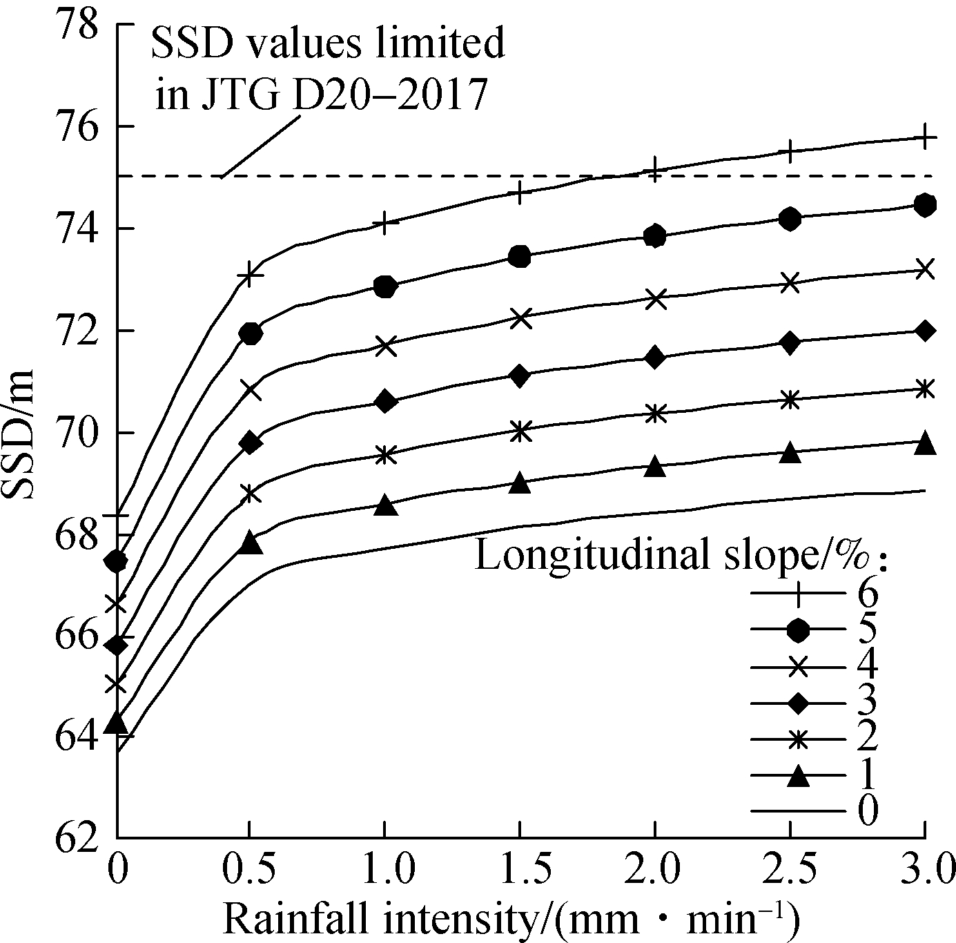
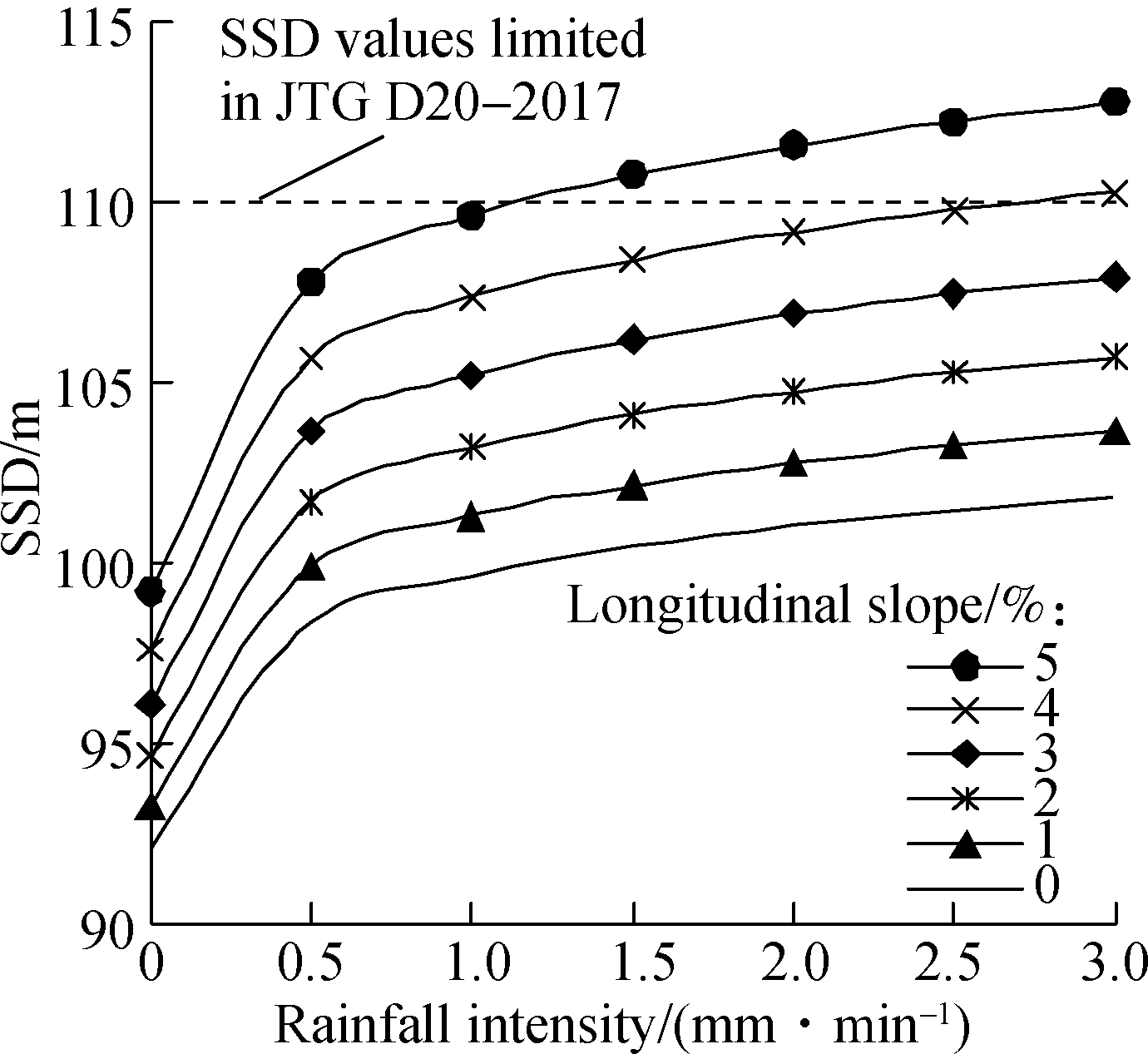
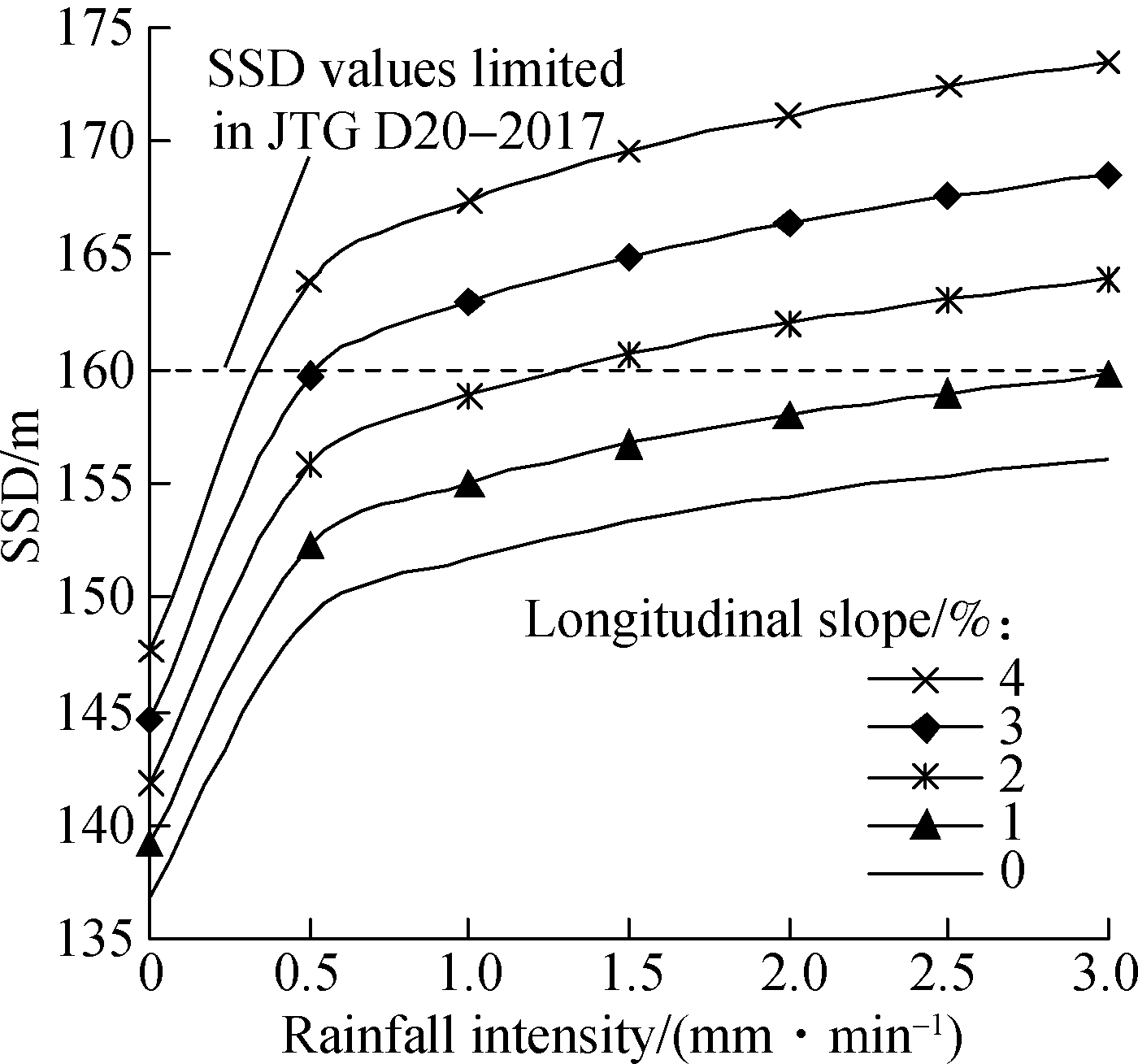
According to the relevant provisions of the Chinese design specification for highway alignment (JTG D20—2017)[7], the SSD values of expressway and first-class highways at different design speeds are shown in Tab.5.
Tab.5 SSD of expressway and first-class highway[7]

Design speed/(km∙h-1)SSD / m120210100160801106075
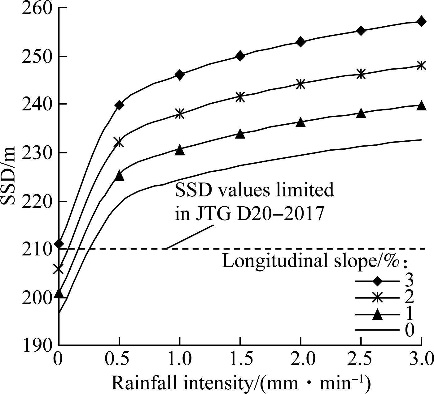
Combining Eqs.(18) and (24) and taking a transverse slope gradient of 2% and Fx=3.75×10⁻⁶ km2 into consideration, the SSD of an asphalt pavement in different regions under wet weather can be calculated. The results for design speeds ranging from 60 to 120 km/h are shown in Fig.7 and can be used as reference values for designers.
Compared with the SSD graphical results of Fig.7, the corresponding values specified in the Chinese design specification for highway alignment[7] are insufficient to satisfy the normal driving safety requirements on rainy days. Therefore, the SSD values should be modified and revised based on different regional rainfall intensities and slopes for optimizing wet-weather safety conditions.
3.4 Wet-weather safe driving-speed determination
According to the wet-weather safe driving model given in Eq.(24), two speed limits are obtained, namely, the speed limits based on SSD limited by highway alignments, and the speed limits based on visibility under rainy conditions. The lower of the two is typically taken as the safe driving speed limit for a specific rainfall intensity. Example results are shown in Tab.6, Tab.7, and Fig.8, respectively.
From the results in Tab.6, Tab.7, and Fig.8, it is noted that the consideration of SSD for highway alignment governs the safe driving speed limit at larger slopes and smaller rainfall intensities. In contrast, the consideration of visibility under rainy weather governs smaller slopes and larger rainfall intensities. Based on the actual pavement skid resistance under different geometric alignments and meteorological conditions, the highway agencies can design the variable speed limit control strategy for each segment of the highway under wet weather conditions.
(a)
(b)
(c)
(d)
Fig.7 Corrected values of SSD for asphalt pavements under different design speeds. (a) V=60 km/h; (b) V=80 km/h; (c) V=100 km/h; (d) V=120 km/h
Tab.6 Safe driving speeds based on visibility km/h

Longitudinalslope/%Rainfall intensity I/(mm∙min-1)0.51.01.52.02.53.0015511896817062115311795807061215011594796961314811393786860414511291776760514311090776759614010889766658
Tab.7 Safe driving speeds based on SSD km/h

Longitudinalslope/%Rainfall intensity I/(mm∙min-1)0.51.01.52.02.53.03969595949494484838382828256968686767676555454545454
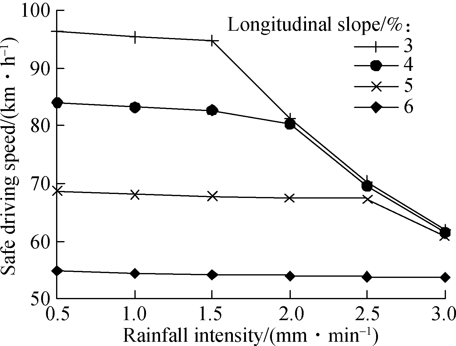
Fig.8 Recommended speed limits for asphalt pavements
4 Conclusions
1) The model for characterizing WFT as a function of rainfall intensity and slope was proposed based on the total discharge formulation and turbulence theory of slope flow in this paper. The proposed model formulation was verified to be reasonable and practical by comparing the predicted WFT with those obtained from empirical formulae and experimental regression models.
2) A WFT model was mathematically formulated as a function of rainfall intensity and slopes (longitudinal and transverse). The model allows for quantifying the WFT under various rainfall intensities and slopes.
3) Regression relationships between BPN and WFT were established based on the experimental data. It is concluded that the BPN value is linearly proportional to the transverse slope and inversely proportional to the rainfall intensity and the longitudinal slope, respectively. Rainfall intensity was found to have a significant impact on the BPN value.
4) The skid resistance characteristics of an asphalt pavement were characterized using the texture depth concept to establish some BPN and SFC60 correlations. Based on these correlations, this paper proposed some BPN and SFC60 values for new asphalt pavements under different rainfall intensities to optimize wet-weather driving safety conditions.
5) The current SSD stipulation in the Chinese codes and specifications is very broad and not regionally specific. As proposed in this paper, the SSD criteria for highways should be revised and modified to be more representative of the prevailing rainfall intensities and slopes. Similarly, the safe driving speed limit control strategy for highways needs enhancements to minimize traffic accidents in wet weather conditions.
As the BPN equation proposed in this paper depended on experimental test data that was restricted to SMA and AC pavements, more pavement types and more skid resistance performance indices are recommended for future studies.
[1]Ivan J N, Ravishanker N, Jackson E, et al. A statistical analysis of the effect of wet-pavement friction on highway traffic safety[J]. Journal of Transportation Safety & Security, 2012, 4(2): 116-136. DOI:10.1080/19439962.2011.620218.
[2]Zhou H C, Wang G L, Yang J, et al. Numerical simulation of effect of bionic V-riblet non-smooth surface on tire anti-hydroplaning[J]. Journal of Central South University, 2015, 22(10): 3900-3908. DOI:10.1007/s11771-015-2934-7.
[3]Luo W T, Li L. Development of a new analytical water film depth (WFD) prediction model for asphalt pavement drainage evaluation[J]. Construction and Building Materials, 2019, 218: 530-542. DOI:10.1016/j.conbuildmat.2019.05.142.
[4]He J C. Effect of texture property on the decreases of skid resistance on wet pavement surface [D]. Nanjing: Southeast University, 2017. (in Chinese)
[5]Kogbara R B, Masad E A, Kassem E, et al. A state-of-the-art review of parameters influencing measurement and modeling of skid resistance of asphalt pavements[J]. Construction and Building Materials, 2016, 114: 602-617. DOI:10.1016/j.conbuildmat.2016.04.002.
[6]Gribbin J E. Introduction to hydraulics and hydrology with applications for stormwater management[M]. 4th ed. New York: Delmar Cengage Learning, 2014.
[7]Ministry of Transport of the People’s Republic of China. JTG D20—2017 Design specification for highway alignment [S]. Beijing: China Communications Press, 2017. (in Chinese)
[8]Taler D. Determining velocity and friction factor for turbulent flow in smooth tubes[J]. International Journal of Thermal Sciences, 2016, 105: 109-122. DOI:10.1016/j.ijthermalsci.2016.02.011.
[9]Ministry of Transport of the People’s Republic of China. JTG/T D33—2012 Specifications for drainage design of highway [S]. Beijing: China Communications Press, 2012. (in Chinese)
[10]Zhao H D, Wu M Z, Wu S T. Variation of asphalt pavement friction coefficient with change of water film thickness [J]. Journal of Civil Aviation University of China, 2015, 33(2): 47-52. DOI:10.3969/j.issn.1674-5590.2015.02.011. (in Chinese)
[11]Veith A G. Tires-roads-rainfall-vehicles: The traction connection [J]. Frictional Interaction of Tire and Pavement, 1983, 793: 3-40. DOI:10.1520/STP28516s.
[12]Ministry of Transport of the People’s Republic of China. JTG D50—2006 Specifications for design of highway asphalt pavement [S]. Beijing: China Communications Press, 2006. (in Chinese)
[13]Hsu C J, Jones E G. Sensitivity analyses of stopping distance for connected vehicles at active highway-rail grade crossings[J]. Accident Analysis & Prevention, 2017, 99: 210-217. DOI:10.1016/j.aap.2016.12.007
[14]Zheng B S, Zhu S Z, Cheng Y Z, et al. Analysis on influence factors of adhesion characteristic of tire-asphalt pavement based on tire hydroplaning model [J]. Journal of Southeast University (Natural Science Edition), 2018, 48(4): 719-725. DOI:10.3969/j.issn.1001-0505.2018.04.019. (in Chinese)
[15]Yin X Q, Zhou F. Measurement of rolling resistance coefficient under vehicle driving conditions [J]. Automotive Technology, 1999(2): 23-25. (in Chinese)
[16]Chu L J, Fwa T F. Pavement skid resistance consideration in rain-related wet-weather speed limits determination [J]. Road Materials and Pavement Design, 2018,19(2):334-352. DOI:10.1080/14680629.2016.1261723.
[17]Zhao L P. Study on traffic safety and control strategy of expressway under the coupling effects of wind and rain [D]. Xi’an: Chang’an University, 2013. (in Chinese)