In many industrial processes, some key process parameters are of great importance to the implementation of control strategies and production plans[1]. However, in some situations, due to the technical problems, a high investment cost or measurement delay, it is difficult to obtain these variables using hardware sensors[2]. To solve this issue, soft sensing technology has been studied and applied by many scholars in the past decades[3-5]. Soft sensor modeling methods can be divided into the mechanism modelling method and data-driven modeling method[6-7]. The mechanism modeling method has the advantages of strongly explanatory and easily understood, but it also has the disadvantages of a complex model and poor portability, especially for some complicated thermal and chemical processes. The other soft sensor modelling method, namely data-driven method, can be developed through learning the historical data. There are various methods applied to setting up data-driven models, for instance, a support vector machine[8], Gaussian process regression[9], artificial neural networks (ANNs)[10], and so on. Compared with other methods, ANNs show prominent advantages due to their good non-linear mapping and generalization ability. Hence, ANNs have been used in a wide variety of industrial process modeling[11-12].
Actually, the accuracy and stability of soft sensor models are the most important criteria to evaluate the quality of models established. In spite of having strong fitting and generalization capability, ANNs are essentially unstable methods based on the statistical theory. The output of ANNs highly depends on the initial weight and training samples. Previous studies also have shown that the performance of a single neural network model is unstable. The performance of ANNs depends heavily on the model structure, especially for the number of nodes and layers in the hidden layers. With the increase in industrial complexity, the dimensionality and coupling of process data tend to be larger, which undoubtedly increases the difficulty of data-driven modelling methods. Hence, some efforts have been made to increase the generalization and stability capability by scholars through various technical methods, for instance, the ensemble method, regularization approach, and so on. Among the above techniques, the ensemble approach seems to be pretty effective. Hansen et al.[13] firstly proposed ANN ensemble in 1990. Many previous studies have confirmed that the neural network ensemble can show better performance for the same issue by aggregating the outputs of some individual neural networks[14]. The reason why the ensemble learning model exhibits a high prediction accuracy is that the ensemble method can balance the outputs of multiple individual subnets, weakening the influence of imperfect models.
Although ANN ensemble approaches have a wide application in practice, one important issue should be considered. General neural network models in ANN ensemble use very time-consuming training methods, such as the back propagation (BP) method to train the model, which suffers from some insuperable disadvantage, such as a plenty of adjustable parameters and danger of over-fitting[15]. To deal with this difficult problem, a kind of effective ANN model called extreme learning machine (ELM) is selected. Different from other neural network methods, ELM transforms the learning training problem into solving the least squares norm problem of the output weight matrix, which gives it the advantages of avoiding falling into local extremism and having a powerful generalization capability[16]. Moreover, many kinds of activation functions can become an ELM inner function, regardless of whether the function is continuous or discontinuous. Due to these advantages, ELM is used to construct an ANN ensemble model in this work. However, the common ELM model uses single type of activation function, which can restrict the performance and robustness of ELM.
To eliminate such restrictions, the heterogeneous ensemble model based on kernel extreme learning machine (KELM) and multiple inner functions of ELMs (HEELM) is developed. In the proposed HEELM ensemble model, five kinds of ELMs (sigmoid activation functions ELM, sin activation functions ELM, radbas activation functions ELM, tribas activation functions ELM and one KELM) are selected as individual models. Meanwhile, to further improve the performance of the ensemble model, least squares regression is used to aggregate the outputs of each signal models. In order to validate HEELM performance, the HEELM is used to establish the soft sensor models of two real-world complex datasets, and simultaneously, unlike other single models. Finally, test results prove that the proposed HEELM has both a good generalization capability and strong robustness.
1 Theory and Algorithm
1.1 ELM
ELM was firstly proposed by Huang et al.[17], and it has been widely applied in various fields in recent years. The structure of the ELM is given in Fig.1, where we can recognize that the ELM is a three-layer neural network. Compared with the traditional BP or RBF network, the ELM model has a relatively fast learning speed, the reasons of which lie in two aspects: One is that the biases and input weights of the ELM are randomly assigned, and the other is that the least square approach is applied to calculate the output weights of the ELM. The procedure of the ELM algorithm is exhibited below.
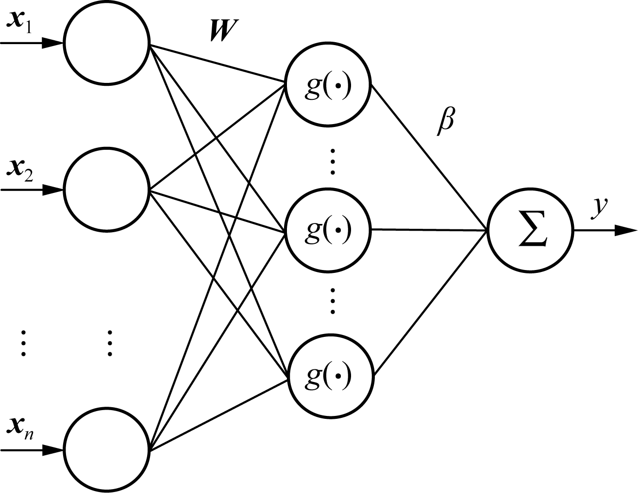
Fig.1 The structure of ELM
Suppose that there are N training samples (xi, ti), in which xi={xi1, xi2,…, xin}T∈Rn, i=1,2,…,N, are the input data and ti=[ti1, ti2,…,tim]T∈Rm, are the output data. n and m are equal to the number of input layer nodes and output nodes of the ELM, respectively. The following form is the computational expression of ELM,
(1)
where βi is the output weights, and it connects the i-th hidden node with the output nodes. Simultaneously, wi represents the input weights, connecting the i-th hidden node with the input nodes; l is the number of hidden layer nodes of the model and g( ·) is the activation function. Previous studies show that the output value of the ELM model can be fitted to samples with zero error. Therefore, a derivation equation can be obtained as
(2)
Eq.(1) can be written as
(3)
Eq.(3) can be simply written as
Hβ=T
(4)
where

(5)
β=[β1,β2,…,βl]T, T=[t1,t2,…,tN]T
(6)
where H is the hidden layer output matrix. In the training process, when wi and bi of ELM are generated, the output matrix H can be obtained, so that the ELM learning training problem is transformed into the least squares norm problem for solving the output weight, and that is
(7)
where H+ is the Moore-Penrose generalized inverse of H.
Hence, the establishment of the ELM model can be achieved by the following four steps:
Step 1 Divide the data sets into two parts: the training data set and testing data set.
Step 2 Randomly assign the input weights and biases and initialize the number of hidden layer nodes.
Step 3 Obtain the output matrix H, and calculate β via training data set.
Step 4 Use the calculated output weights β to calculate the output value of the model with the testing data set.
Obviously, the learning procedure of the ELM is very fast and easy to implement. Nevertheless, there are still some deficiencies when the ELM is used in practice, which are shown as the following three factors: 1) The performance of a single ELM model tends to be affected by the randomly assigned set input weights and biases. 2) An ELM model is only assigned with one activation function, limiting the robustness of the model to a certain extent. 3)When dealing with very complex large-scale data with high collinearity, one standard ELM always shows poor generalization performance.
1.2 Kernel ELM
The kernel ELM (KELM) was proposed by Huang et al.[18] based on the analysis of the support vector machine theory, and it is an extension of the extreme learning machine method. The KELM uses Mercer’s conditions to define kernel matrix Ω and replaces random matrix HHT in the ELM with the kernel matrix Ω,
ΩKELM=HHT, Ωi,j=h(xi) ·h(xj)=K(xi,xj)
(8)
According to the above formula, the output of the KELM model is as
(9)
The KELM method does not need to assign the initial input weights and biases as well as the number of hidden layer nodes. The specific form of the kernel function K(xi, xj) is the unique parameter that needs to be adjusted. In this paper, the radial basis function is selected as the kernel function,
(10)
1.3 Least square regression
Least squares regression (LSR) is an effective linear statistical regression modeling method. Assume that the data set consists of an input (independent) variable X∈Rn×m and an output (dependent) variable Y∈Rn×1 and both variables are mean-centered and scaled by the standard deviation. The linear relationship between the input and output variables is expressed in the matrix form as
Y=X×W+E
(11)
where W is the regression coefficient vector, and E is the residual error matrix.
The optimal linear regression relationship between the input and output variables can be estimated by the least squares algorithm, assuming that the optimal linear relationship obtained by least squares is
(12)
![]() can be calculated as
can be calculated as
(13)
2 Proposed Heterogeneous HEELM Model
To establish a more accurate and stable model for soft sensor modeling, a novel heterogeneous ELM ensemble model called HEELM is developed in this work. The structure diagram of the HEELM is presented in Fig.2. The proposed HEELM model uses five kinds of ELM to enhance the diversity of the individual model, which also can tackle the problem of noise in training data. As shown in Fig.2, sigmoid, sin, rabas, tribas function ELM, as well as KELM are applied for the individual model of the HEELM, and the least squares regression method is used as the aggregation strategy to obtain better ensemble outputs. The detailed steps of the HEELM modeling method are described as follows.
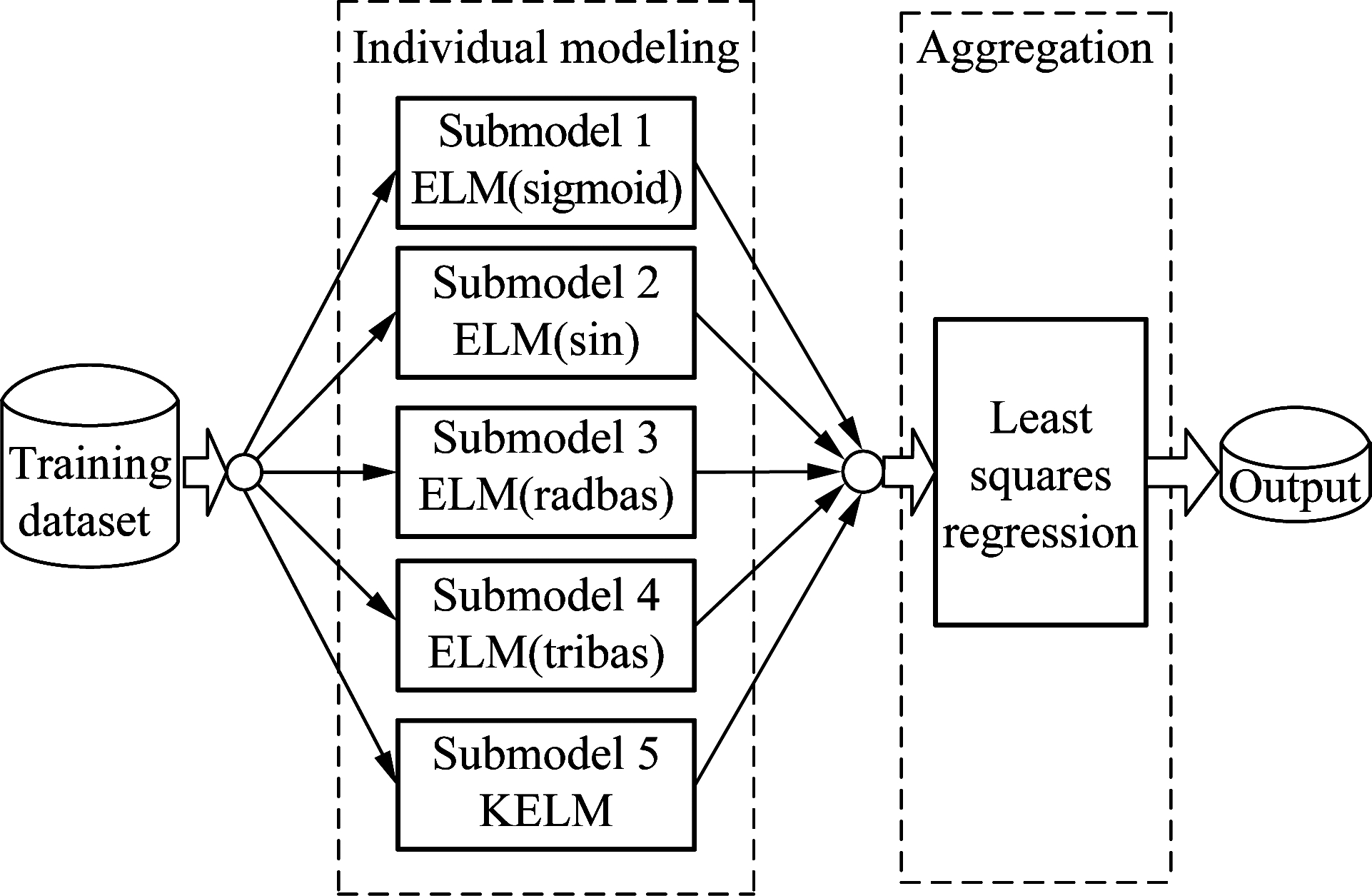
Fig.2 The structure of the HEELM model
Suppose that the data set is D={(Xi, Yi)|i=1,2,…,N}, where Xi=[xi1,xi2,…,xim]∈Rm represents the input data with m variables in Xi; Yi∈R represents output data. Before building the model, the data is divided into three groups: training set Dtr={(Xt, Yt)|t=1,2,…,Ntr}, validation set Dva={(Xv, Yv)|v=1,2,…,Nva}, and testing set Dte={(Xt′, Yt′)|t′=1,2,…,Nte},N=Nte+Nva+Ntr. The validation set is used to validate the number of hidden layer nodes, the ELM models, and C,γ values of KELM.
Step 1 Preprocess input and output data in the same order of amplitude by the following equations:
(14)
(15)
where ![]() are the maximum and minimum of input data. Similarly, Ymax, Ymin are the maximum and minimum of output data, respectively.
are the maximum and minimum of input data. Similarly, Ymax, Ymin are the maximum and minimum of output data, respectively.
Step 2 Set the input weights and biases of ELM models with sigmoid, sin, rabas, tribas activation functions and build individual models using training set. The KELM model does not need to set input weights and other parameters. γ in the kernel function and regularization coefficient C are the two parameters in KELM that need to be optimized. In the present study, two parameters are determined by k-fold cross-validation. Specifically, the training samples are divided into k groups equally. Then, the k-1 groups are used to train the KELM model, and the remaining group is applied to the test model. After k repeated experiments, each group of data can be used as test data in turn. The average of the total test errors is taken as an assessment criterion to evaluate the parameters of the KELM model. Moreover, the most suitable number of hidden nodes of ELM models with sigmoid, sin, rabas, tribas functions is calculated using the trial-and-error approach.
Step 3 Through the training set Dtr, the outputs of five individual sub ![]() are obtained, which are the training output values of five sub-models in Fig.2, respectively.
are obtained, which are the training output values of five sub-models in Fig.2, respectively.
Step 4 Calculate the output of the proposed HEELM model through establishing a regression model between the outputs of each individual model and the expected outputs by the least squares regression technique.
(16)
Step 5 Through the testing set Dte, the outputs of five individual sub ![]() are obtained. Then, the prediction of HEELM model is calculated using the coefficient obtained in Eq.(16).
are obtained. Then, the prediction of HEELM model is calculated using the coefficient obtained in Eq.(16).
(17)
Step 6 To accurately evaluate the performance of the proposed HEELM, the root mean square error (RMSE) is used as evaluation criteria. RMSE can be calculated as
(18)
3 Case Studies
The ensemble model capability is validated using two practical industrial processes: One is the debutanizer and the other is selective catalytic reduction (SCR) flue gas denitration process of the power plant boiler.
3.1 Debutanizer column
The debutanizer column is a part of desulfurization and naphtha splitting plant. Its task is to reduce the concentration of tower bottom butane as much as possible[19]. The flowchart of a debutanizer column process is shown in Fig.3. Usually, the concentration of bottom butane is measured on-line by a gas chromatography analyzer installed on the top of the tower. Since it takes a certain time for the vapor of bottom butane to reach the top of the tower and the analysis process of the gas chromatography analyzer, there is a lag in the on-line measurement of the concentration of bottom butane. So, it is necessary to establish a soft sensor model to estimate the concentration of bottom butane on-line and in real time. There are in total seven variables selected as input variables in the soft sensing model. The only output variable is the concentration of butane in the bottom of the debutanizer. Tab.1 lists the detail description of input variables. There is a total of 2 393 data samples in the debutanizer column process, of which about half are used as training sets, about one-third are test sets and the rest are validation sets. All the data can be downloaded in Ref.[20].
Tab.1 Input variables of soft sensor for the debutanizer column
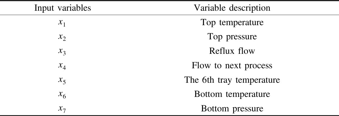
Input variablesVariable descriptionx1Top temperaturex2Top pressurex3Reflux flowx4Flow to next processx5The 6th tray temperaturex6Bottom temperaturex7Bottom pressure

Fig.3 The flowchart of the debutanizer column
In this study, some kinds of single ELM models include ELM with sigmoid, sin, radbas, tribas activation functions, and the KELM model are built to be compared with the HEELM model. To ensure fair comparison, some parameters for five single models such as the number of hidden layer nodes, C and γ are firstly selected by the trial-and-error method. Those parameters can be determined when the errors are the smallest within the validation data.
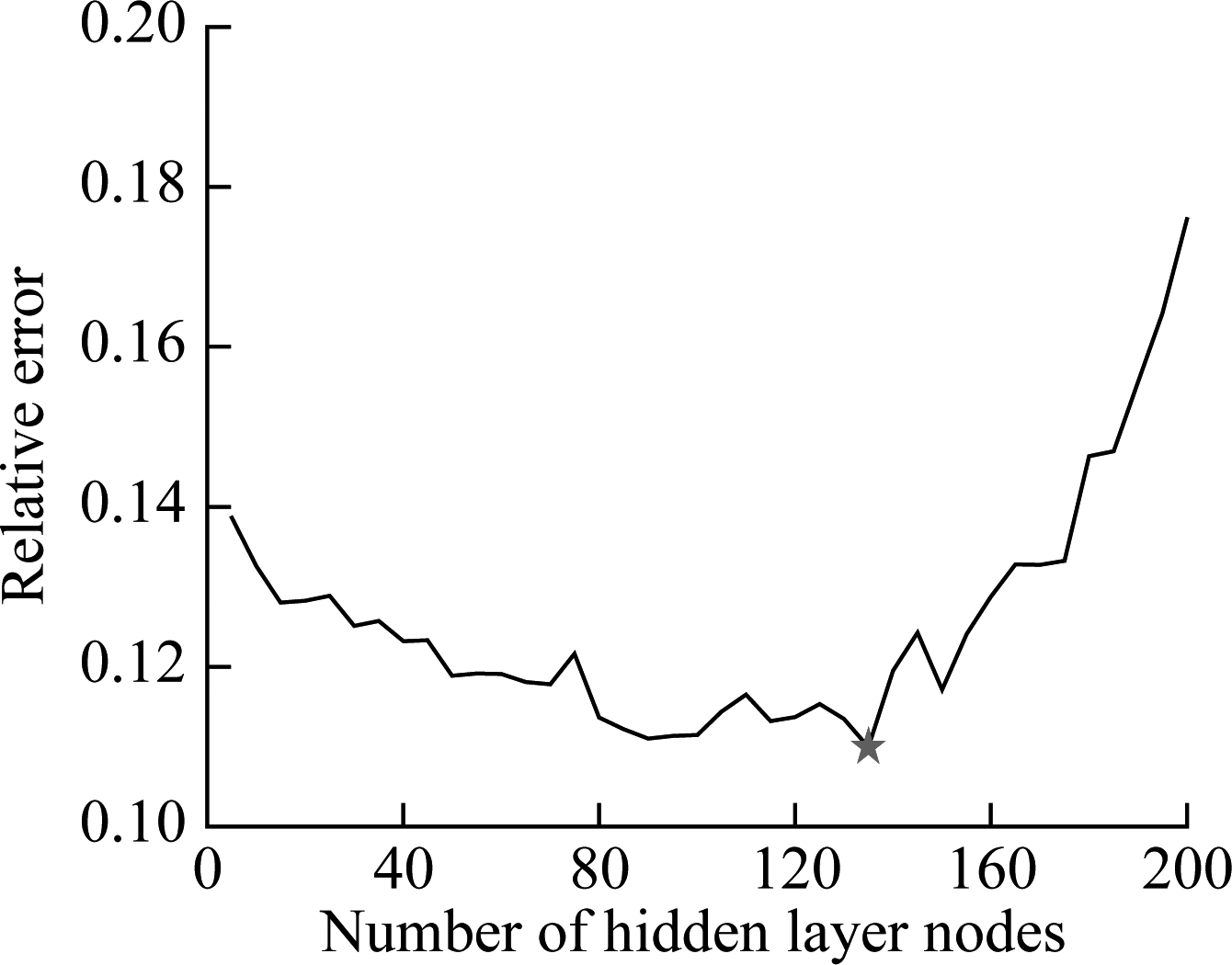
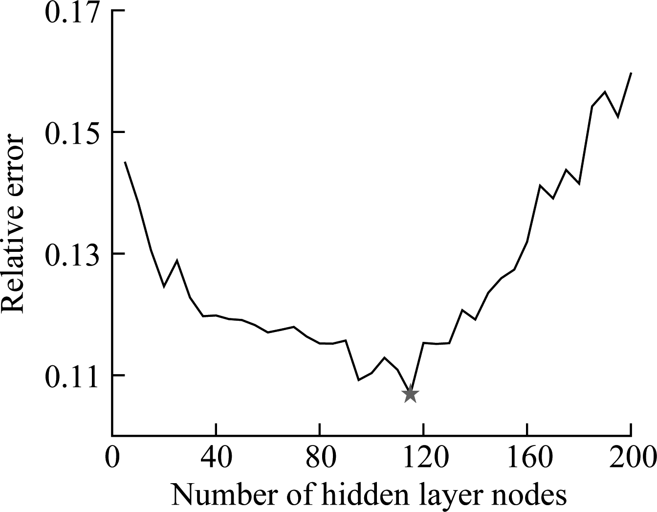
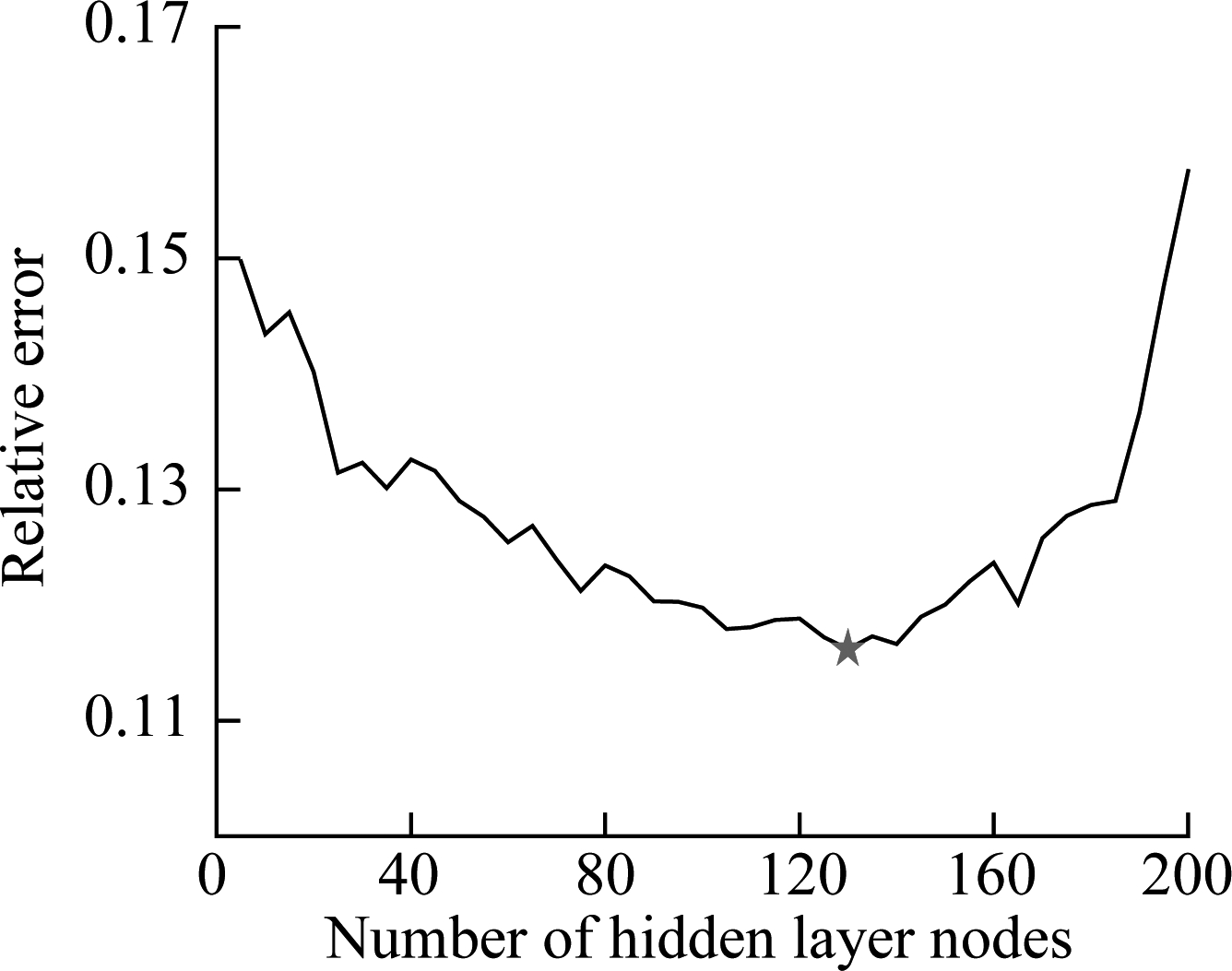
Fig.4 shows the variation of relative errors of the validation set with the number of hidden layer nodes of ELM models. It can be seen that, for the ELM with sigmoid function, the relative error is the least when the number of nodes is 135. Hence, the number of hidden layer nodes of the individual ELM with the sigmoid function is assigned as 135. Similarly, the numbers of hidden layer nodes of single ELM models with sin, radbas, and tribas inner functions are determined as 115, 130 and 130, respectively. In addition, parameters C and γ in the KELM model are finally optimized to be C=50 and γ=0.06. After determining the optimal parameters of each sub-model, the proposed HEELM can be developed via aggregating the outputs of five individual models using the least squares regression strategy. To enhance the reliability of the simulation experiment, the experiment is repeated 30 times, and the max, min, mean and standard deviation (SD) of RMSE values for the testing dataset are shown in Tab.2. Bagging the ELM uses five different ELMs as sub-models. Bagging ensemble is a common ensemble technique, and in this study, the Bagging ELM ensemble model is established to make a comparison with the performance of the proposed HEELM.
As seen from Tab.2, the proposed HEELM model can achieve smaller max, min, and mean of RMSE for the testing dataset than those of the other five individual models and the Bagging ELM model. Fig.5 displays the variation of RMSE values obtained by the seven models in 30 runs for testing the dataset of debutanizer column. It is clear that, the RMSE value of each ELM models with sigmoid, sin, radbas, tribas activation functions varies from 0.086 9 to 0.110 7 with a large fluctuation. The reason for such a result is that although the optimal number of nodes for each ELM model has been determined, the input weights and bias values of the four ELM models are randomly determined in each simulation experiment, which can lead to the unstable prediction performance of the four models. When the optimum parameters (C,γ) are determined, the KELM model has no other parameters that can be adjusted, so the error results of the KELM model for 30 times are invariable. The RMSE values of the HEELM are low and stable around 0.086 0 without fluctuation.
Tab.2 Simulation results of RMSE values for debutanizer column testing dataset
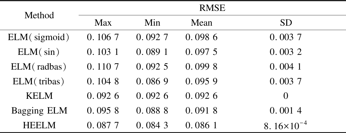
MethodRMSEMaxMinMeanSDELM(sigmoid)0.106 70.092 70.098 60.003 7ELM(sin)0.103 10.089 10.097 50.003 2ELM(radbas)0.110 70.092 50.099 80.004 1ELM(tribas)0.104 80.086 90.095 90.003 7KELM0.092 60.092 60.092 60Bagging ELM0.095 80.088 80.091 80.001 4HEELM0.087 70.084 30.086 18.16×10⁻⁴
(a)

(b)
(c)
(d)
Fig.4 Variation of relative errors of validation set with the number of nodes of ELMs for the debutanizer column. (a) ELM (sigmoid); (b) ELM(sin); (c) ELM(radbas); (d) ELM(tribas)
Apparently, the HEELM model can achieve much better stability than that of single ELM. In addition, the predictive performance of the KELM model is better than that of other four single ELM models, but not as good as that of the HEELM model. The simulation results of the debutanizer column demonstrate that the proposed HEELM model can achieve better prediction accuracy and model stability.
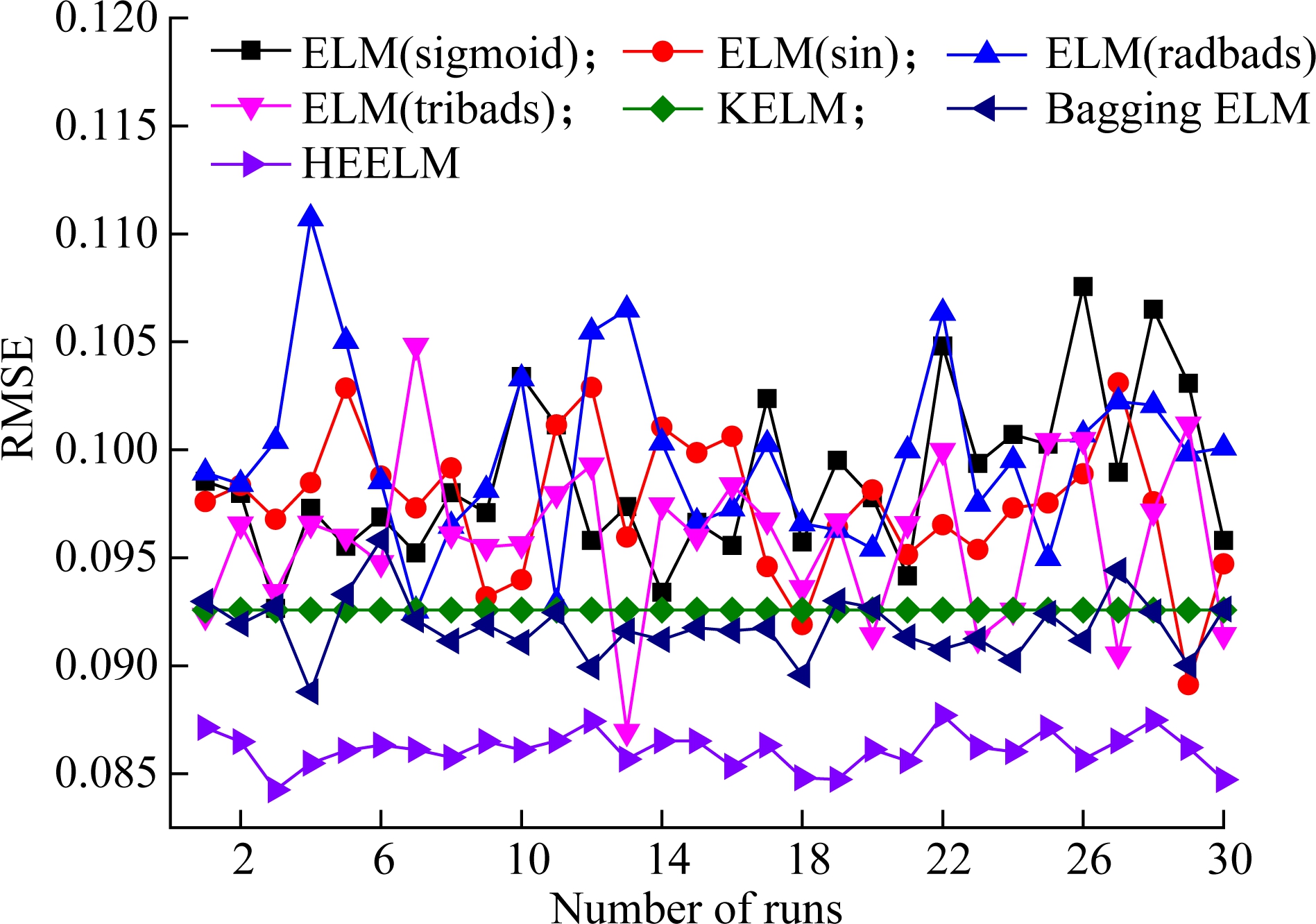
Fig.5 RMSE values for debutanizer column testing dataset of six models
3.2 SCR flue gas denitration process
SCR flue gas denitrification is a necessary technique in coal-fired power plants for reducing the nitrogen oxides (NOx). SCR denitrification technique has some salient features such as high denitrification efficiency and simple device structure, so SCR denitrification has attracted much attention and wide application in almost all power plants. The flowchart of SCR flue gas denitration is shown in Fig.6. The working principle of SCR is that, liquid ammonia reacts with the NOx, and converts NOx to N2 and H2O.
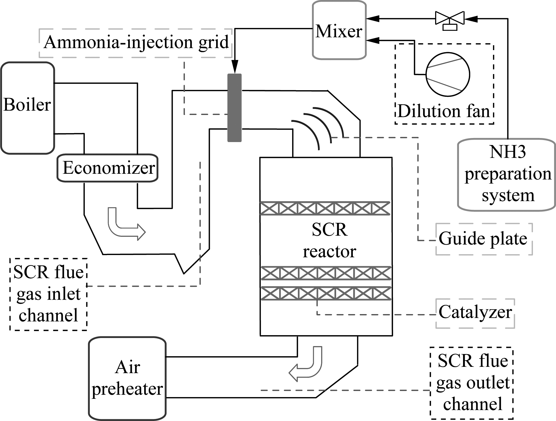
Fig.6 Schematic diagram of reactor structure in SCR flue gas denitrification system
In this work, 1 000 measurements of a 1 000 MW ultra-supercritical boiler SCR denitrification system boiler operation are obtained from the distributed control system (DCS) database. The sampling interval is 1 min. Based on the basic knowledge of boilers and the engineers’ experience [21], six variables are employed as inputs of the SCR model and the only output is the export NOx of the SCR denitrification system. The detailed description of input variables is listed in Tab.3. To construct the soft sensor model, 1 000 samples are divided into three parts: 500 samples are used as training sets, 200 samples are the validation sets and the remaining 300 samples are the test sets.
Tab.3 Input variables of the soft sensor for the SCR flue gas denitration process

Input variablesVariable descriptionx1Entrance NOx concentration x2Inlet gas flow value x3Inlet flue gas temperaturex4Ammonia injection x5Unit loadx6Entrance O2 concentration
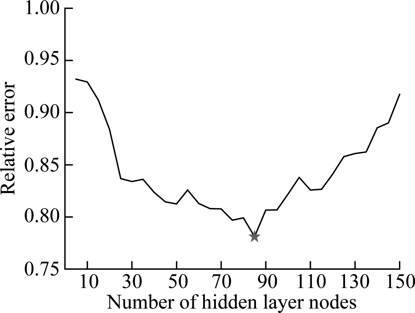
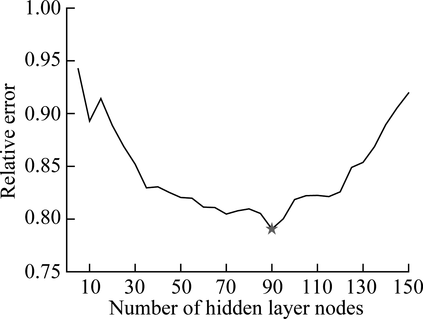
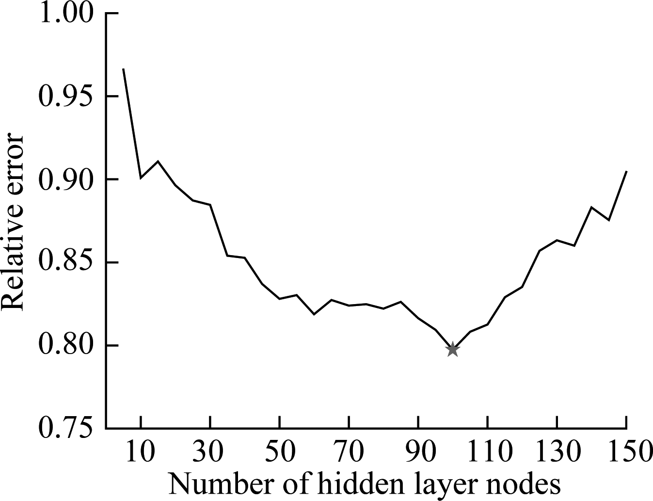
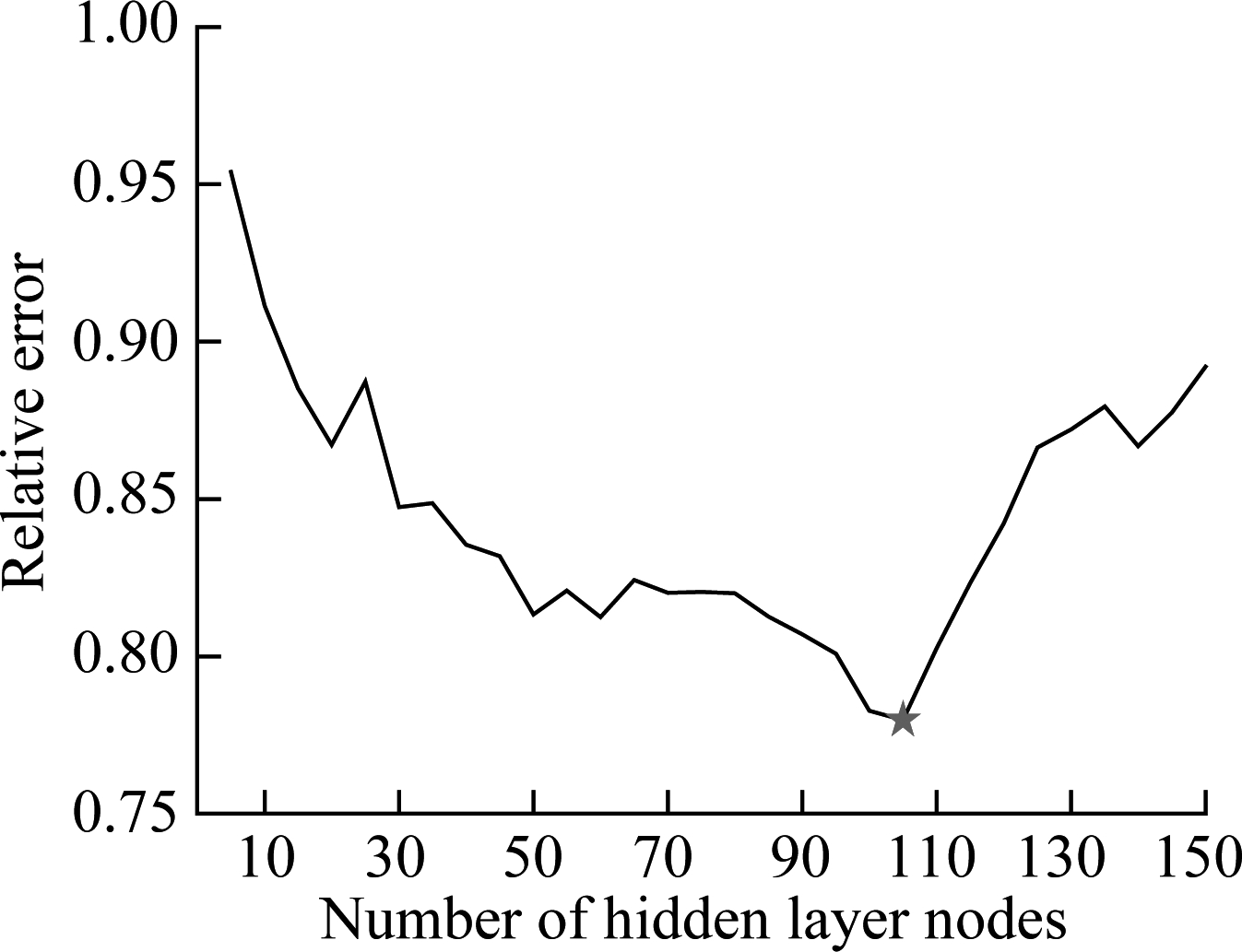
According to the steps of the proposed HEELM approach mentioned above, the number of hidden layer nodes of four common ELM with different activation functions and two parameters (C,γ) of KELM are firstly determined. Similar to the number of hidden layer nodes determination of debutanizer column simulation in section 3.1, Fig.7 presents the relative errors of the validation set with the number of ELM models’ nodes. It can be seen from Fig.7 that, for the SCR flue gas denitration dataset, the most suitable number of hidden layer nodes for four ELM models with sigmoid, sin, radbas, tribas functions is assigned as 85, 90, 100 and 105, respectively. Moreover, according to the cross validation method, C and γ in the KELM model are assigned to be 50 and 0.1, respectively.
After 30 repeated experiments, the results of the soft model for SCR flue gas denitration case are listed in Tab.4. Compared with the five single ELM models, BP model and SVM model, it can be clearly seen that the HEELM method can obtain smaller REME values. The SD values of RMSE four common ELM models with sigmoid, sin, radbas, tribas activation functions and BP model are obviously higher than that of the HEELM model, which reveals that the common single ELM model is unstable. Meanwhile, the HEELM model combines the outputs of five ELM models to solve the problem that includes the complex data. Five different kinds of ELM models can realize mutual complementation by least square technique when establishing the soft sensor model. Therefore, the proposed HEELM ensemble model can show the highest accuracy among all the presented models.
To further show the capability of the HEELM method, a comparison between the predicted results and real data of 300 testing cases is presented in Fig.8. The red line is the perfect line which shows that predicted values are equal to real values, and the points are the results predicted by the HEELM method. It is easy to see that all of the points distribute closely around the perfect line, which means that the output is the export NOx of SCR which can be predicted with good accuracy by the proposed HEELM for the testing dataset. Moreover, in order to clearly show the generalization performance of six kinds of ELMs, Fig.9 presents the variation of RMSE values obtained by the eight models in 30 runs for testing the dataset of SCR flue gas denitration. From Fig.9, it can be seen that the RMSE values of HEELM are the smallest in all 30 times experiments. Hence, all the simulation re-sults of SCR flue gas denitration indicate that the HEELM ensemble model can achieve a high accuracy and good stability.
(a)
(b)
(c)
(d)
Fig.7 Schematic diagram of reactor structure in SCR flue gas denitrification system. (a) ELM(sigmoid); (b) ELM(sin); (c) ELM(radbas); (d) ELM(tribas)
Tab.4 Simulation results of RMSE values for SCR flue gas denitration testing dataset
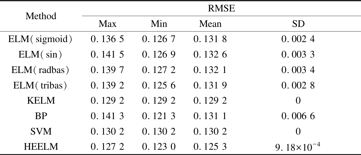
MethodRMSEMaxMinMeanSDELM(sigmoid)0.136 50.126 70.131 80.002 4ELM(sin)0.141 50.126 90.132 60.003 3ELM(radbas)0.139 70.127 20.132 10.003 4ELM(tribas)0.139 20.125 60.131 90.002 8KELM0.129 20.129 20.129 20BP0.141 30.121 30.131 10.006 6SVM0.130 20.130 20.130 20HEELM0.127 20.123 00.125 39.18×10⁻⁴
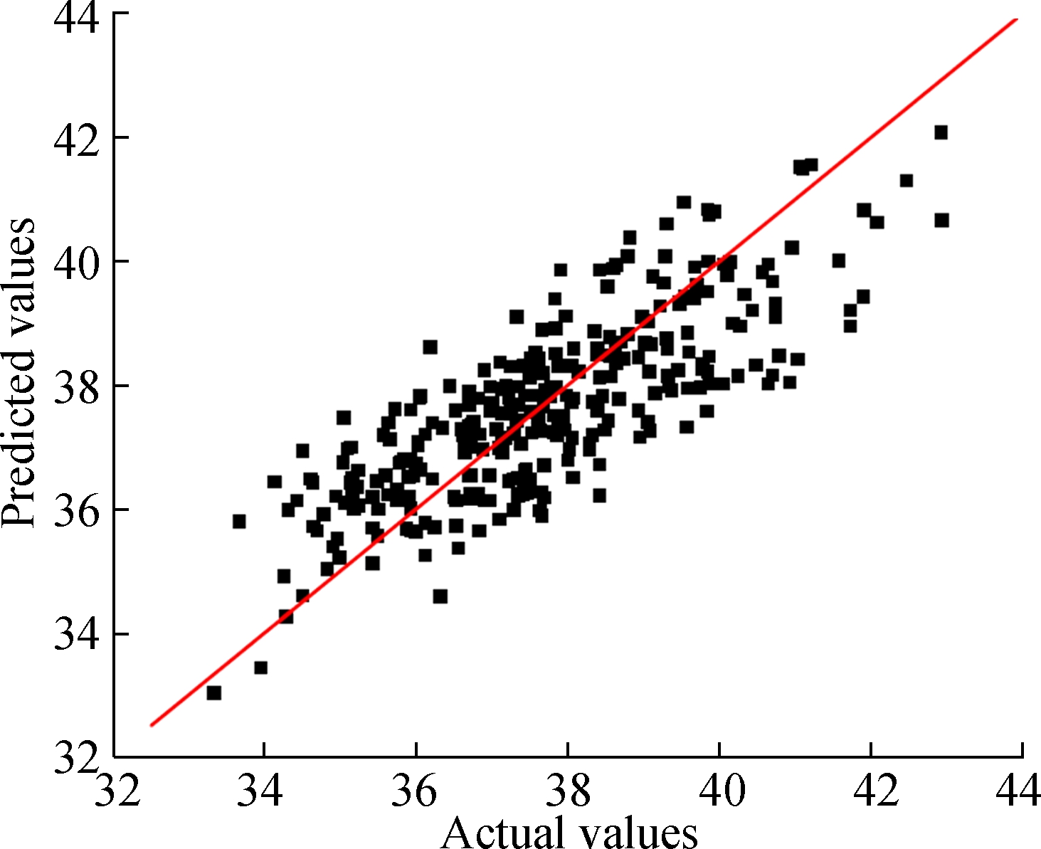
Fig.8 Fitting performance of the HEELM model for SCR flue gas denitration testing dataset
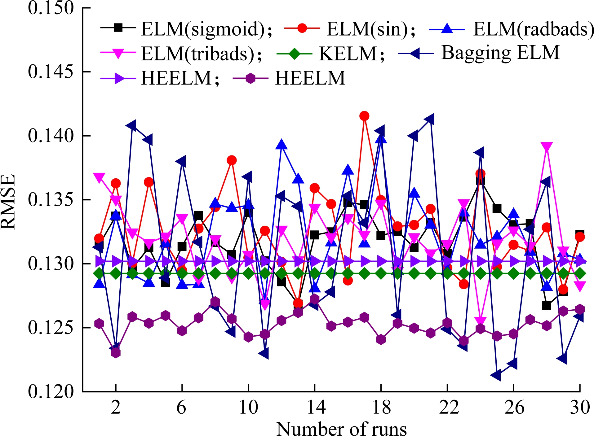
Fig.9 RMSE values for SCR flue gas denitration testing dataset of eight models
4 Conclusions
1) An advanced approach for soft sensor modeling using a heterogeneous ensemble, namely HEELM, is proposed. Five kinds of ELM algorithms are used for obtaining diversity within the HEELM model in handling complex modeling data. The least square method is used as an effective ensemble technique to enhance the generalization ability by ensuring the worst individual model have the least impact on the final output.
2) The generalization performance of the proposed HEELM ensemble model is verified by two real datasets from the debutanizing and the SCR flue gas denitration processes. The simulation results show that the HEELM model can achieve a good performance in generalization accuracy and stability.
3) The modeling performance of the HEELM is also compared with individual ELM models, bagging ELM ensemble model, BP, as well as SVM models, and the results demonstrate that the perfomance of HEELM is better than that of the other models in the aspects of its predictive accuracy.
4) In future study work, other kinds of aggregating techiques and different neural network ensemble models will be studied and utilized.
[1]Wang T, Gao H J, Qiu J B. A combined adaptive neural network and nonlinear model predictive control for multirate networked industrial process control[J]. IEEE Transactions on Neural Networks and Learning Systems, 2016, 27(2): 416-425. DOI:10.1109/tnnls.2015.2411671.
[2]Yuan X F, Ge Z Q, Song Z H. Soft sensor model development in multiphase/multimode processes based on Gaussian mixture regression[J]. Chemometrics and Intelligent Laboratory Systems, 2014, 138: 97-109. DOI:10.1016/j.chemolab.2014.07.013.
[3]Zheng J H, Song Z H. Semisupervised learning for probabilistic partial least squares regression model and soft sensor application[J]. Journal of Process Control, 2018, 64: 123-131. DOI:10.1016/j.jprocont.2018.01.008.
[4]Popli K, Afacan A, Liu Q, et al. Development of online soft sensors and dynamic fundamental model-based process monitoring for complex sulfide ore flotation[J]. Minerals Engineering, 2018, 124: 10-27. DOI:10.1016/j.mineng.2018.04.006.
[5]Sun Y M, Wang Y L, Liu X G, et al. A novel Bayesian inference soft sensor for real-time statistic learning modeling for industrial polypropylene melt index prediction[J]. Journal of Applied Polymer Science, 2017, 134(40): 45384. DOI:10.1002/app.45384.
[6]Wang F F, Li P F, Mi J C, et al. A refined global reaction mechanism for modeling coal combustion under moderate or intense low-oxygen dilution condition[J]. Energy, 2018, 157: 764-777. DOI:10.1016/j.energy.2018.05.194.
[7]Bala Subramaniyan A, Pan R, Kuitche J, et al. Quantification of environmental effects on PV module degradation: A physics-based data-driven modeling method[J]. IEEE Journal of Photovoltaics, 2018, 8(5): 1289-1296. DOI:10.1109/jphotov.2018.2850527.
[8]Wang X X, Hu H L, Jia H Q, et al. SVM-based multisensor data fusion for phase concentration measurement in biomass-coal co-combustion[J]. Review of Scientific Instruments, 2018, 89(5): 055106. DOI:10.1063/1.5007100.
[9]Ge Z Q. Active probabilistic sample selection for intelligent soft sensing of industrial processes[J]. Chemometrics and Intelligent Laboratory Systems, 2016, 151: 181-189. DOI:10.1016/j.chemolab.2016.01.003.
[10]Li G Q, Chen B, Chan K C C, et al. Modeling thermal efficiency of a 300 MW coal-fired boiler by online least square fast learning network[J]. Journal of Chemical Engineering of Japan, 2018, 51(1): 100-106. DOI:10.1252/jcej.17we114.
[11]Mohanraj M, Jayaraj S, Muraleedharan C. Applications of artificial neural networks for refrigeration, air-conditioning and heat pump systems: A review[J]. Renewable and Sustainable Energy Reviews, 2012, 16(2): 1340-1358. DOI:10.1016/j.rser.2011.10.015.
[12]Naveen Kumar V, Lakshmi Narayana K V. Development of thermistor signal conditioning circuit using artificial neural networks[J]. IET Science, Measurement & Technology, 2015, 9(8): 955-961. DOI:10.1049/iet-smt.2015.0008.
[13]Hansen L K, Salamon P. Neural network ensembles[J]. IEEE Transactions on Pattern Analysis and Machine Intelligence, 1990, 12(10): 993-1001. DOI:10.1109/34.58871.
[14]Pham B T,Shirzadi A, Tien Bui D, et al. A hybrid machine learning ensemble approach based on a Radial Basis Function neural network and Rotation Forest for landslide susceptibility modeling: A case study in the Himalayan area, India[J]. International Journal of Sediment Research, 2018, 33(2): 157-170. DOI:10.1016/j.ijsrc.2017.09.008.
[15]Samiee K, Iosifidis A, Gabbouj M. On the comparison of random and Hebbian weights for the training of single-hidden layer feedforward neural networks[J]. Expert Systems with Applications, 2017, 83: 177-186. DOI:10.1016/j.eswa.2017.04.025.
[16]Li G Q, Niu P F, Duan X L, et al. Fast learning network: a novel artificial neural network with a fast learning speed[J]. Neural Computing and Applications, 2014, 24(7/8): 1683-1695. DOI:10.1007/s00521-013-1398-7.
[17]Huang G B, Zhu Q Y,Siew C K. Extreme learning machine: Theory and applications[J]. Neurocomputing, 2006, 70(1/2/3): 489-501. DOI:10.1016/j.neucom.2005.12.126.
[18]Huang G B, Wang D H,Lan Y. Extreme learning machines: A survey[J]. International Journal of Machine Learning and Cybernetics, 2011, 2(2): 107-122. DOI:10.1007/s13042-011-0019-y.
[19]Fortuna L,Graziani S, Xibilia M G. Soft sensors for product quality monitoring in debutanizer distillation columns[J]. Control Engineering Practice, 2005, 13(4): 499-508. DOI:10.1016/j.conengprac.2004.04.013.
[20]Shao W M. Research on adaptive soft sensing modeling method based on local learning [D]. Qingdao: China University of Petroleum, 2016. (in Chinese)
[21]Wu X, Shen J, Sun S Z, et al. Data-driven disturbance rejection predictive control for SCR denitrification system[J]. Industrial & Engineering Chemistry Research, 2016, 55(20): 5923-5930. DOI:10.1021/acs.iecr.5b03468.