The hybrid test, first proposed by Hakuno in 1969, is an effective test technique which combines a physical loading experiment and numerical simulation to evaluate seismic responses of large complex civil structures. At present, it has been widely focused on by researchers, and certain research results have been achieved such as a numerical integration algorithm[1-2], real time hybrid test[3], loading control[4], time delay compensation[5], boundary condition[6], remote network collaborative hybrid test[7], and an accurate numerical element[8], etc. The hybrid test has been widely used in the test of large and complex civil structures[9-10]. However, when the hybrid test is conducted on large complex structures, it is impossible to perform a physical loading test on all critical parts. Thus, some key components or parts of the structure are modeled and analyzed in the numerical substructure. Due to model errors, the inaccuracy of the numerical simulation will increase when the entire structure enters nonlinearity. The two main reasons for model errors are: 1) The assumed numerical model is too simple to describe the nonlinear behaviors of the real structure or component; 2) The uncertainty of model parameters. When the proportion of the assumed numerical models with model errors become larger, the accuracy of hybrid tests will be reduced. Therefore, how to improve the model accuracy and restore the force prediction accuracy of the numerical substructure has become an urgent problem.
Model updating is an effective method to improve the accuracy of hybrid tests, which has been widely used in finite element analysis over the past two decades. The theory of model updating can be specified as follows: In the process of hybrid tests, the data of the experimental substructures can be used to recognize and update the numerical model of numerical substructures with similar hysteresis behaviors. Therefore, the model errors of the numerical substructure are reduced, and the ability to predict the structural actual behaviors is improved.
1 Principle of Model Updating in Hybrid Tests
As shown in Fig.1, the model updating hybrid test consists of four parts, namely the numerical integration module, the experimental loading module, the assumed restoring force model module and the model updating module. It can be seen from the figure that the restoring force of the experimental substructure RE,k+1 can be obtained by inputting the displacement command  into the model updating module in the model updating hybrid test. In the model updating module, the data from the experimental substructure is applied to identify and update the numerical model of the numerical substructures with similar hysteresis behaviors. Many computational methods are applied to model updating to achieve better accuracy, such as parameter identification methods[8-14], intelligent algorithms[15-16],etc.

Fig.1 Procedure of model updating hybrid test
Among all the parameter identification methods, the initial selected numerical model is usually simplified from the experimental results, which means that the limited number of parameters cannot fully describe the real nonlinear behaviors. In other words, the model gap between the simplified model and the real model exists from the early beginning of the hybrid tests. In contrast, the intelligent algorithms can acquire more hysteresis information that does not exist in the initial assumed numerical model, and can directly fit the constitutive model of the numerical substructure. Therefore, the intelligent algorithms address the shortcomings of the parameter identification methods. However, in intelligent algorithms, the BP neural network has a poor generalization ability and it is relatively sensitive to initial weight, which will influence the accuracy of the constitutive model.
In order to solve the problem of poor generalization ability and sensitivity to the initial weight of the BP neural network, an online AdaBoost regression tree algorithm is proposed and adopted. First, some weak regressors are selected for training; then the multiple weak regressors are integrated into a strong regressor; and finally the training results are generated. In order to verify the effectiveness of the proposed model updating method, a numerical simulation of a 2-DOF nonlinear structure is carried out, and the results are compared with the BP neural network algorithm.
2 Principle of Regression Tree Algorithm
The regression tree is a type of decision tree for regression. A decision tree is a tree-like model defined in the feature space, as shown in Fig.2. The regression tree algorithm proposed by Breiman et al.[17] mainly includes two steps: regression tree generation and regression tree pruning.
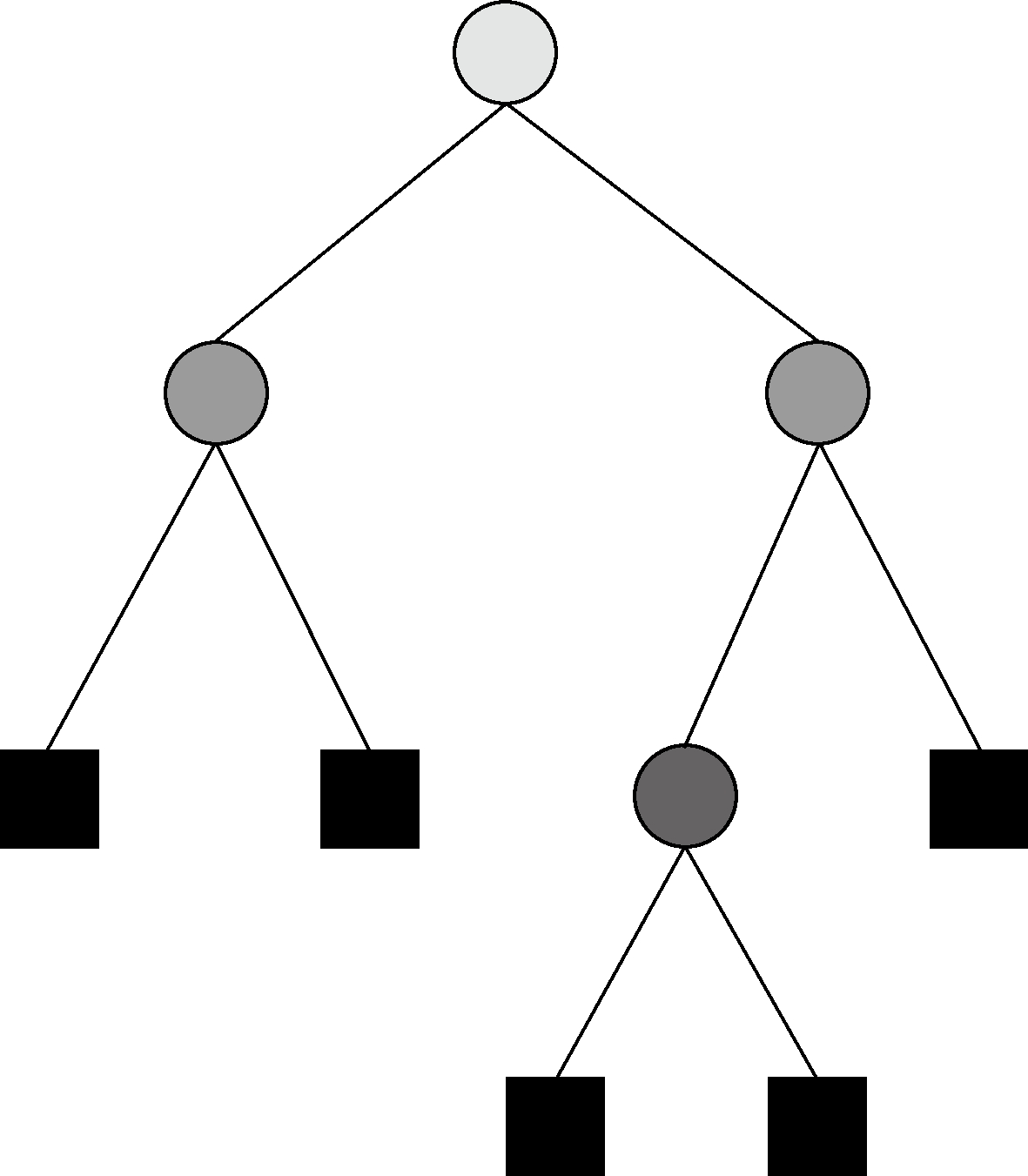
Fig.2 The regression tree model diagram
2.1 Regression tree generation
The regression tree model consists of nodes and directed edges as shown in Fig.2. The nodes include internal nodes and leaf nodes. The circles and boxes in Fig.2 represent internal nodes and leaf nodes, respectively. The internal nodes represent the characteristics or attributes of the samples, and the leaf nodes represent the prediction value of the samples. The least squares algorithm is used to generate the regression tree. The specific process is as follows:
It is supposed that x and y denote the input and output variables, respectively, and the training data set is D={(x1,y1),(x2,y2),…,(xN,yN)}. The input space is divided into M regions, namely, R1,R2,…,Rm,…,RM and each region Rm has a fixed output value cm. Thus, the regression tree model can be expressed as
(1)
where the optimal value of cm is set to be ![]() which is the average value of output value yi in region Rm.
which is the average value of output value yi in region Rm.
(2)
The heuristic algorithm is used to segment the input space. The j-th variable x(j) and the corresponding value s are selected as the split variable and split point, respectively. The next two regions are defined as
R1(j,s)={x|x(j)≤s}, R2(j,s)={x|x(j)>s}
(3)
Then, the best split variable x(j) and the split point s are searched for by solving the minimum value:
(4)
The best split points in R1(j,s) and R2(j,s) are as follows:
(5)
After all the input variables (j,s) are traversed, the optimal partition variable x(j) is established and the input space is divided into two regions one by one. Next, the above segmentation process is repeated for each region until the stop condition is reached. Thus, a regression tree is generated.
2.2 Regression tree pruning
In order to prevent the over fitting of the above-mentioned regression tree model, it is necessary to prune the generated regression tree to ensure its generalization ability. The pruning algorithm performs recursive pruning according to the principle of loss function minimizing, including the following two steps:
From the bottom of the regression tree T0 to the top, pruning is continued until the procedure reaches the root nodes. Then, a pruned subtree sequence {T0,T1,…,Tn} is formed and the loss function of the subtrees during pruning is calculated as follows:
Cα(T)=C(T)+α|T|
(6)
where T is an arbitrary subtree; C(T) is the prediction error of the training data; |T| is the number of leaf nodes in a subtree; and the parameter α(α≥0) measures the fitting degree of the training samples and the complexity of the model. Cα(T) indicates the entire loss of the subtree T when the parameter is α. The pruning process is repeated till the root node.
Based on the validation data set, the cross validation method is used to test the subtree sequence obtained from the above process. Also, the optimal subtree Tα is obtained based on the independent verification data set. The decision tree with the smallest square error in the subtree sequence {T0,T1,…,Tn} is selected as the optimal one. The pruning diagram of the regression tree is illustrated in Fig.3
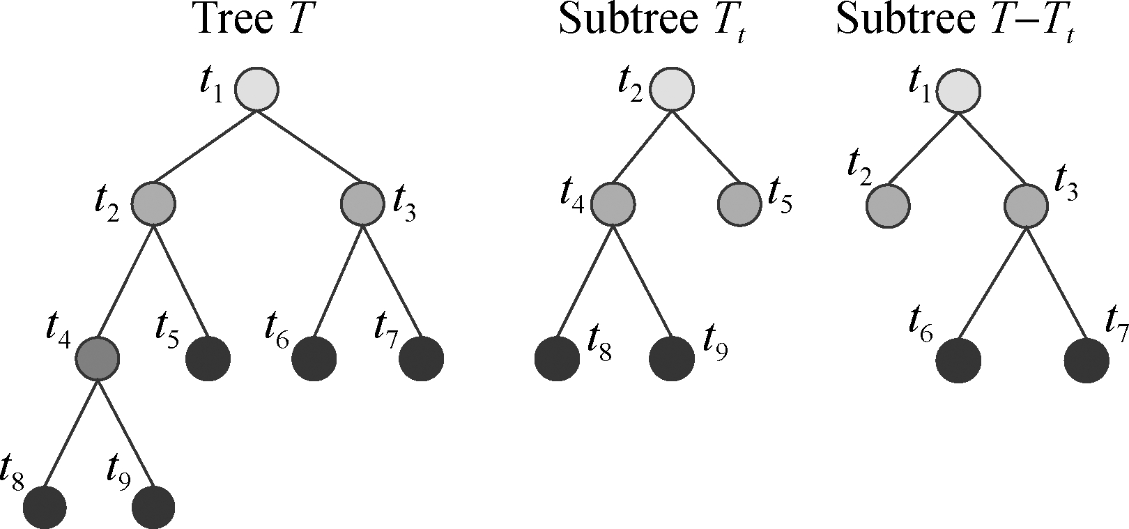
Fig.3 The regression tree pruning diagram
3 Implementation of online AdaBoost regression tree algorithm
For the constitutive model recognition of the nonlinear components, large generalization errors cannot be avoided when only one neural network model is adopted for training. The training results of multiple neural network models are more accurate than those of the single neural network model, which is called the boosting method. The representative boosting method is the AdaBoost algorithm proposed by Freund and Schapire[18] in 1995. Firstly, the regression tree is selected for training and the weight of each training sample is adjusted in each round of training. Then, these regression tree models are integrated linearly to vote out the final results. The diagram of the Adaboost regression tree algorithm is shown in Fig.4.
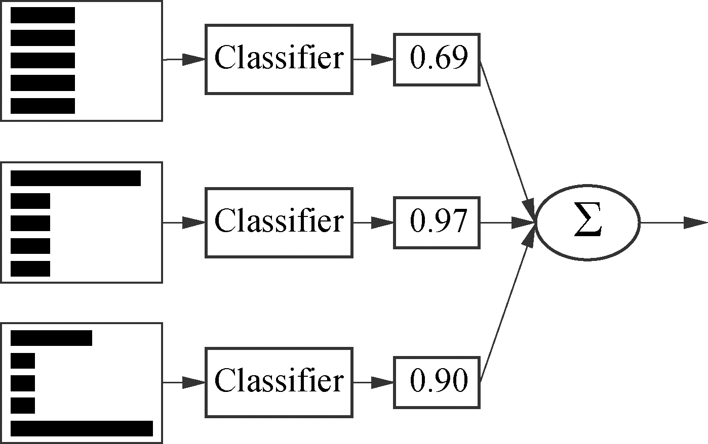
Fig.4 The diagram of Adaboost regression tree algorithm
In hybrid tests, the samples of the experimental substructure in the current step are input into the Adaboost regression tree model for training, and a strong regressor is obtained. Then, after inputting the displacement of the numerical substructure in the current step into the trained strong regressor, the corresponding restoring force can be directly predicted. The procedure based on the proposed method is illustrated in Fig.5.
3.1 Collecting training samples
After establishing the equation of motion of the entire structure, the numerical integration scheme is applied to solve the equation to obtain the displacements of the experimental substructure and numerical substructure in the i-th step, which are defined as  of the experimental substructure in the i-th step are extracted as the training samples to train the AdaBoost regression tree model online.
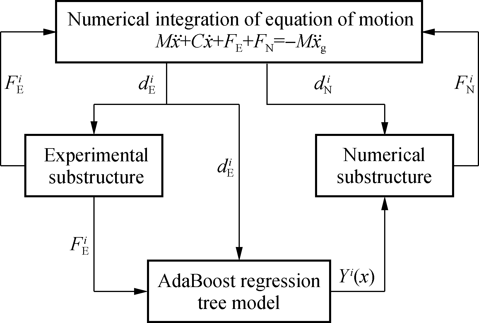
Fig.5 Procedure based on the proposed method in hybrid test
3.2 Weight initialization of training samples
In the first loading step, the initial weight of training samples is set to be
(7)
where ![]() N is the number of training samples.
N is the number of training samples.
In the i-th step, the initial weight vector of the training samples is set to be the weight vector trained after M iterations in the (i-1)-th step:
(8)
where M denotes the number of iterations and M is set to be 20 in this paper. ![]() is the weight vector of the training samples trained after M iterations in the i-th step.
is the weight vector of the training samples trained after M iterations in the i-th step.
3.3 Training AdaBoost regression tree model
In each loading step in the model updating hybrid test, M iterations are executed to train the AdaBoost regression tree model. In the m-th iteration (m=1,2,…,m,…,M), the initial weight vector of training samples at the m-th iteration are set as the trained weight vector in the (m-1)-th iteration. In the i-th loading step, the regression tree in the m-th iteration is trained to obtain the regressor ![]()
The updating criterion of the training sample weight is: If the regression error of a certain sample point is small, the weight of this sample will be reduced in the next iteration; on the contrary, if the regression error of a certain sample point is large, the weight of this sample will be increased in the next iteration. Following the learning rule of the AdaBoost regression tree algorithm, the weight of unpredictable samples is increased and the prediction accuracy of the restoring force is finally improved. The training process mainly includes the following steps.
1) Calculate the regression error of ![]() at the m-th iteration:
at the m-th iteration:
(9)
2) Calculate the weight coefficient of ![]()
(10)
When ![]() decreasing, it means that, in the final prediction, the decisive role of the regression tree model becomes larger while the regression error becomes smaller.
decreasing, it means that, in the final prediction, the decisive role of the regression tree model becomes larger while the regression error becomes smaller.
3) The weight of the training samples is updated in each iteration. The update rules are
(11)
(12)
(13)
where ![]() is the normalization factor, which makes the sum of the weight coefficients 1.0.
is the normalization factor, which makes the sum of the weight coefficients 1.0.
3.4 Combining regression tree models
The M regression tree models are linearly integrated into a strong regressor Yi(x) in the i-th step:
(14)
The diagram of integrating regression tree models is shown in Fig.6.
3.5 Prediction of restoring force in hybrid tests
The restoring force of the numerical substructure in the i-th step can be predicted by inputting the displacement into the integrated regressor obtained above. Then, the restoring force of the experimental substructure and numerical substructure are fed back to the equation of motion. The five steps are repeated until the ground motion input is completed.
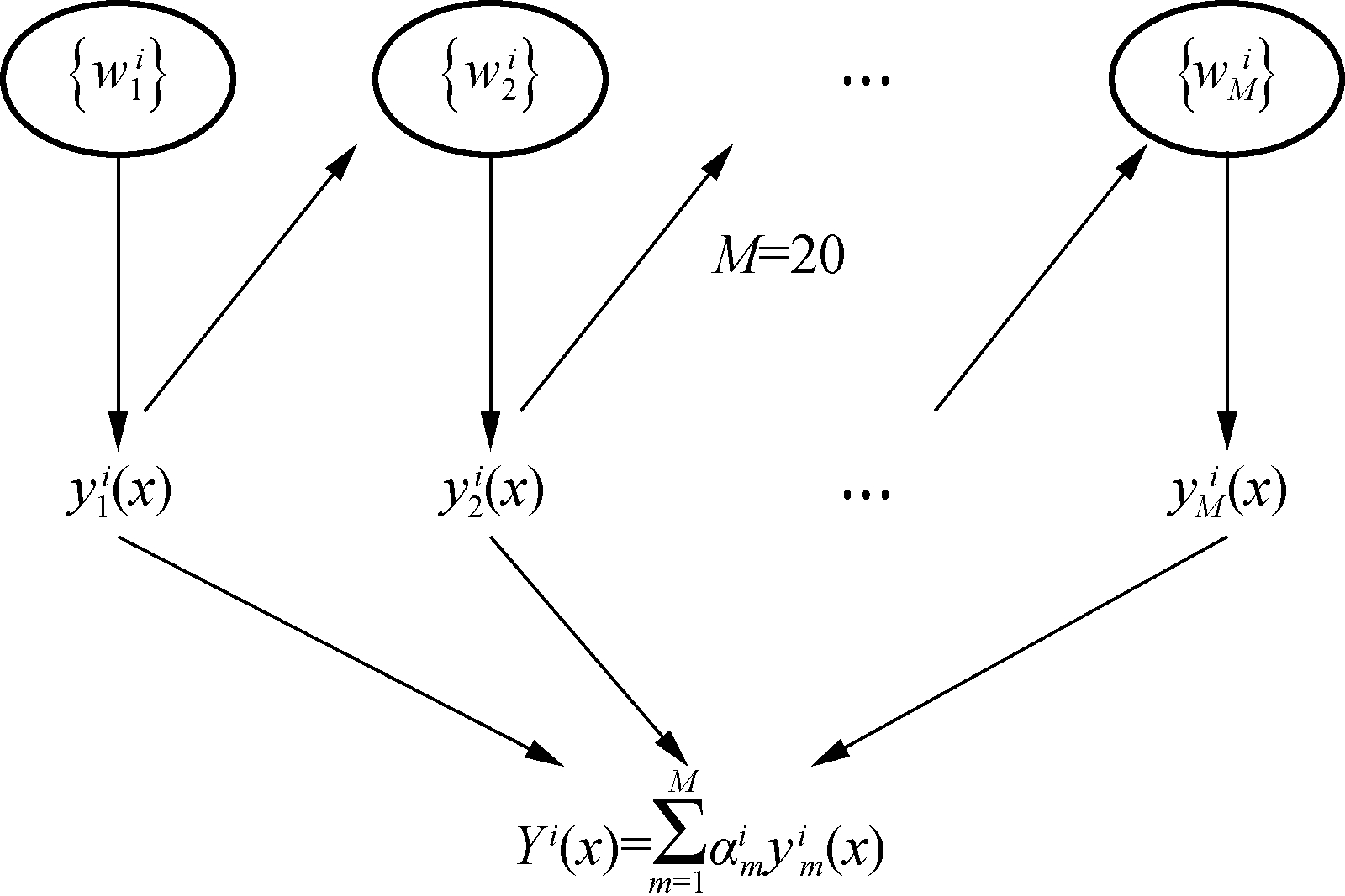
Fig.6 The diagram of integrating regression tree models
4 Numerical Validation
4.1 Model description
The online AdaBoost regression tree algorithm is evaluated on a 2-DOF nonlinear structure as shown in Fig.7. It is assumed that there are no complex incomplete boundaries and no obvious different loading histories.
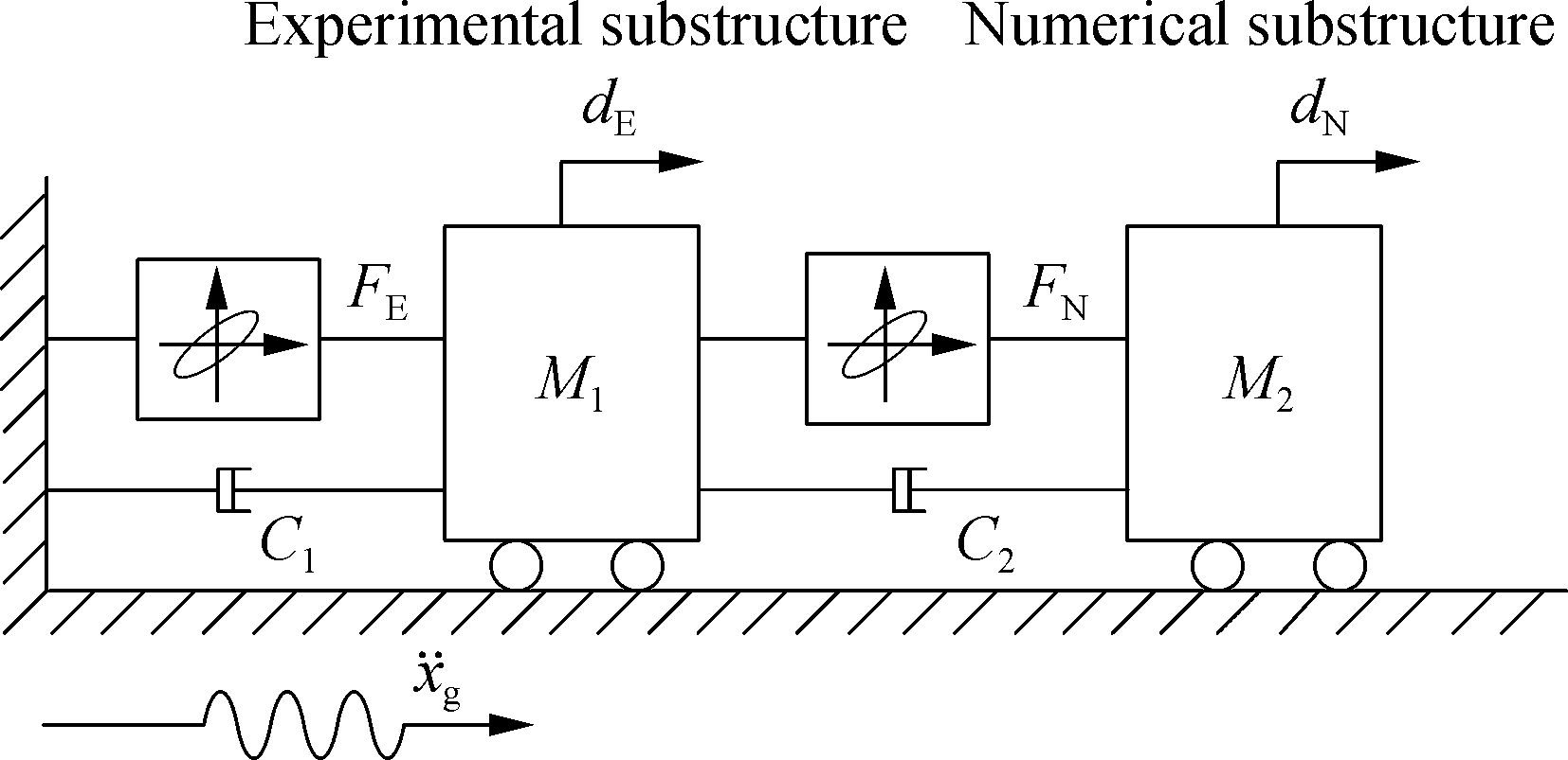
Fig.7 A 2-DOF nonlinear structure model
The masses of the experimental substructure and numerical substructure are M1=M2=2 500 t; the initial stiffnesses are K1=K2=394 785 kN/m; and the damping coefficients are C1=C2=5 026.5 kN/(m·s-1). The ground motion recorded at the SimiValley-Katherine Rd station on January 17, 1994 at the Northridge earthquake is selected for numerical simulation. The peak seismic acceleration is adjusted to 200 cm/s2. The Runge-Kutta method is applied as the numerical integration scheme and the sample time is set to be 0.01 s. In this numerical study, it is assumed that the real constitutive models of the experimental substructure and numerical substructure are both the Bouc-Wen model, that is
(15)
where F is the restoring force of the structure; α is the second stiffness coefficient; K is the initial stiffness of the structure; Z is the hysteretic displacement; and β, γ, n are the model parameters that control the shape of the hysteresis curve. The real model parameters of the experimental substructure and numerical substructure in this numerical study are both set to be as follows: K=394 785 kN/m, α=0.01, A=1, β=100, γ=40, n=1.
The input variables of the nonlinear hysteresis model are set to be 6 variables as follows:di,di-1,Fi-1,Fi-1di-1,Fi-1Δdi and Ei-1. di is the relative displacement of the structure in the i-th step; Δdi=di-di-1; Fi-1 is the restoring force of the structure in the i-th step; Fi-1di-1 is the energy consumption of the structure in the (i-1)-th step; Fi-1Δdi is the energy consumption of structure in the i-th step; Ei-1[19]is the cumulative energy consumption of the structure in the (i-1)-th step, Ei-1=Ei-2+|Fi-1di-1|.
4.2 Results analysis
In order to verify the effectiveness of the proposed method, three types of hybrid tests are analyzed and compared in this numerical simulation, as shown in Figs.8 and 9. The reference in the figures represents the true hybrid test; the BP algorithm in the figures represents the model updating hybrid test based on the BP neural network algorithm; the AdaBoot algorithm in the figures represents the hybrid test of model updating based on the AdaBoot regression tree algorithm.
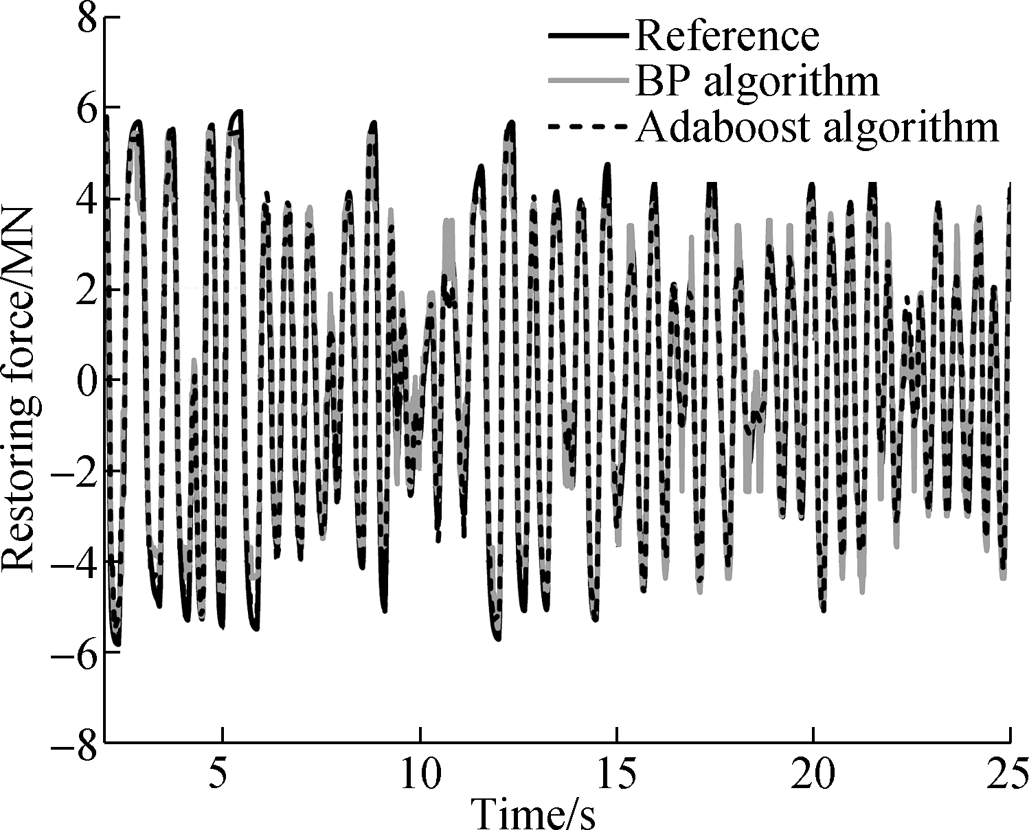
Fig.8 Comparison of the restoring force prediction of the numerical substructure with online AdaBoost regression tree and BP neural network algorithm
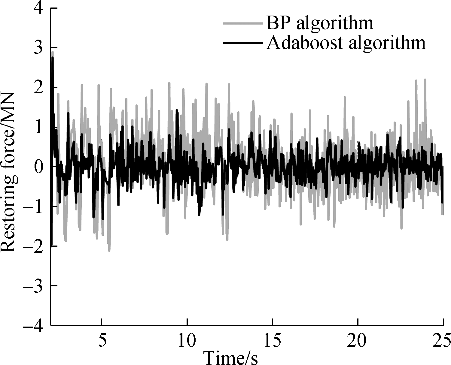
Fig.9 Comparison of the restoring force prediction error of the numerical substructure with an online AdaBoost regression tree and BP neural network algorithm
Fig.8 and Fig.9 show the comparison of restoring force prediction error and restoring force prediction error of the numerical substructure in three simulation cases, respectively. It can be seen from Fig.8 that the restoring force of the numerical substructure predicted by the AdaBoost regression tree algorithm is in good agreement with the real value, while the restoring force predicted by the BP algorithm has a large error at the turning point.
Fig.9 shows that the maximum absolute error of the predicted restoring force based on the BP neural network algorithm is larger than that of the AdaBoost regression tree algorithm on the whole. The AdaBoost regression tree algorithm gradually adapts to the new data through online training and reduces the prediction error of the restoring force over time.
In order to quantify the prediction error of the restoring force, the dimensionless error index is utilized in this study. The root mean deviation (RMSD) is
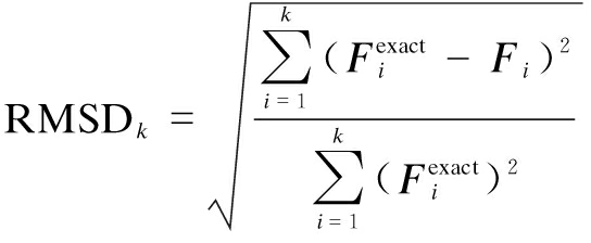
(16)
where ![]() denotes the true restoring force of the structure in the i-th step; and Fi is the predicted restoring force of the structure in the i-th step. Fig.10 shows the RMSD comparison between the BP neural network algorithm and the AdaBoost regression tree algorithm.
denotes the true restoring force of the structure in the i-th step; and Fi is the predicted restoring force of the structure in the i-th step. Fig.10 shows the RMSD comparison between the BP neural network algorithm and the AdaBoost regression tree algorithm.
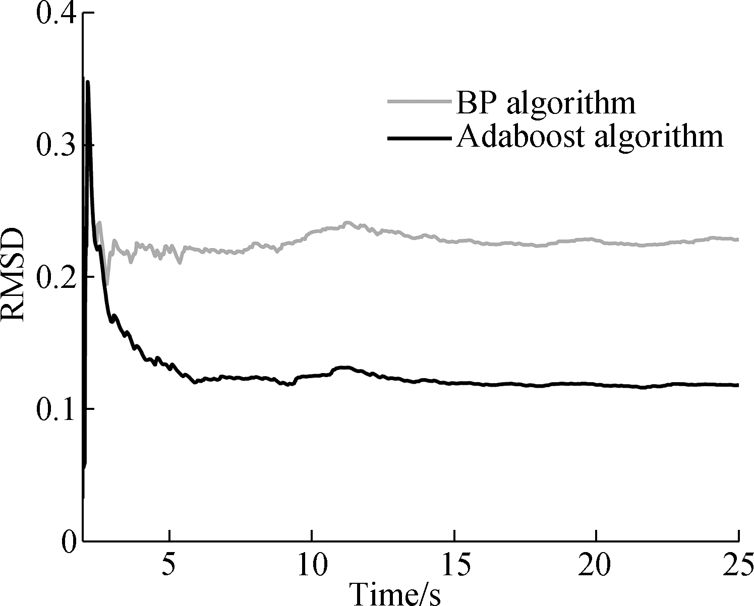
Fig.10 Comparison of the RMSD with the online AdaBoost regression tree and BP neural network algorithm
It can be seen from Fig.10 that in the initial stage of hybrid tests, the prediction errors of the BP neural network algorithm and AdaBoost regression tree algorithm are relatively large. However, as time goes on, the prediction errors of the restoring force in both cases gradually decrease and tend to stabilize.
In the stable stage, the RMSD of the online AdaBoost regression tree algorithm is 0.117 9, and that of the BP neural network algorithm is 0.228 2. The prediction accuracy of the online AdaBoost regression algorithm is 48.3% higher than that of the BP neural network algorithm. In addition, the average one-step time of the proposed method is 0.12 s, which meets the requirements of slow hybrid tests. Therefore, the method proposed in this paper can significantly improve the model accuracy in hybrid tests, and has reference value for the application of intelligent algorithms to the hybrid test of model updating.
5 Conclusion
1) The numerical analysis of a 2-DOF nonlinear structure is conducted to verify the effectiveness of the proposed method.
2) Compared with the online BP neural network algorithm, the absolute error of the restoring force prediction is reduced by 72.5% and the relative root mean square error is reduced by 48.3% when the online AdaBoost regression tree algorithm is adopted, which verifies the effectiveness of the proposed method.
3) The generalization ability of the recognition system is improved. The research results are significant for the application of intelligent algorithms to improve the model accuracy in a hybrid test.
[1] Wu B, Xu G S, Wang Q, et al. Operator-splitting method for real-time substructure testing [J]. Earthquake Engineering & Structural Dynamics, 2006, 35(3): 293-314. DOI: 10.1002/eqe.519.
[2] Wu B, Bao H, Ou J, et al. Stability and accuracy analysis of the central difference method for real-time substructure testing [J]. Earthquake Engineering & Structural Dynamics, 2005, 34(7): 705-718. DOI:10.1002/eqe.451.
[3] Nakashima M, Kato H, Takaoka E. Development of real-time pseudo dynamic testing [J]. Earthquake Engineering & Structural Dynamics, 1992, 21(1): 79-92. DOI:10.1002/eqe.4290210106.
[4] Wang Z, Wang Z R, Yang J, et al. Secondary development of MTS control system and its application to hybrid tests [J]. Earthquake Engineering and Engineering Dynamics, 2015, 35(2): 22-29. DOI:10.13197/j.eeev.2015.02.22.wangz.003. (in Chinese)
[5] Xu W J, Guo T, Chen C. Research in parameter α of inverse compensation for real-time hybrid simulation [J]. Engineering Mechanics, 2016, 33(6): 61-67. DOI:10.6052/j.issn.1000-4750.2014.12.1075. (in Chinese)
[6] Wu B, Ning X Z, Xu G S, et al. A novel hybrid simulation method considering incomplete boundary conditions [J]. Journal of Vibration and Shock, 2018, 37(15): 150-155. DOI:10.13465/j.cnki.jvs.2018.15.021. (in Chinese)
[7] Kwon O S, Elnashai A S, Spencer B F. A framework for distributed analytical and hybrid simulations [J]. Structural Engineering and Mechanics, 2008, 30(3): 331-350. DOI:10.12989/sem.2008.30.3.331.
[8] Chuang M C, Hsieh S H, Tsai K C, et al. Parameter identification for on-line model updating in hybrid simulations using a gradient-based method [J]. Earthquake Engineering & Structural Dynamics, 2018, 47(2): 269-293. DOI:10.1002/eqe.2950.
[9] Yang Y S, Tsai K C, Elnashai A S, et al. An online optimization method for bridge dynamic hybrid simulations [J]. Simulation Modelling Practice and Theory, 2012, 28: 42-54. DOI:10.1016/j.simpat.2012.06.002.
[10] Wang T, Wu B, Zhang J. Online identification with least square method for pseudo-dynamic tests [J]. Advanced Materials Research, 2011, 250/251/252/253:2455-2459. DOI:10.4028/www.scientific.net/amr.250-253.2455.
[11] Hashemi M J, Masroor A, Mosqueda G. Implementation of online model updating in hybrid simulation [J]. Earthquake Engineering & Structural Dynamics, 2014, 43(3): 395-412. DOI:10.1002/eqe.2350.
[12] Wang T, Wu B. Hybrid testing method based on model updating with constrained unscented Kalman filter [J]. Journal of Earthquake Engineering and Engineering Vibration, 2013, 33(5): 100-109. DOI:10.13197/j.eeev.2013.05.100.wangt.013. (in Chinese)
[13] Wu B, Wang T. Model updating with constrained unscented Kalman filter for hybrid testing [J]. Smart Structures and Systems, 2014, 14(6): 1105-1129. DOI:10.12989/sss.2014.14.6.1105.
[14] Ou G, Dyke S J, Prakash A. Real time hybrid simulation with online model updating: An analysis of accuracy [J]. Mechanical Systems and Signal Processing, 2017, 84: 223-240. DOI:10.1016/j.ymssp.2016.06.015.
[15] Elanwar H H, Elnashai A S. Framework for online model updating in earthquake hybrid simulations [J]. Journal of Earthquake Engineering, 2016, 20(1): 80-100. DOI:10.1080/13632469.2015.1051637.
[16] Wang T, Zhan X H, Meng L Y. Hybrid testing method based on an online neural network algorithm [J]. Journal of Vibration and Shock, 2017, 36(14): 1-8. DOI:10.13465/j.cnki.jvs.2017.14.001. (in Chinese)
[17] Breiman L, Friedman J, Stone C J, et al. Classification and regression trees [M]. Boca Raton, FL, USA: CRC Press, 1984.
[18] Freund Y, Schapire R E. A decision-theoretic generalization of on-line learning and an application to boosting [C]// Proceedings of the Second European Conference on Computational Learning Theory. Berlin: Springer-Verlag, 1995: 23-27. DOI:10.1007/3-540-59119-2_166.
[19] Kim J, Ghaboussi J, Elnashai A S. Hysteretic mechanical-informational modeling of bolted steel frame connections [J]. Engineering Structures, 2012, 45: 1-11. DOI:10.1016/j.engstruct.2012.06.014.