In recent years, there has been a significant amount of progress in developing intelligent transportation system(ITS)applications and services such as automated vehicle navigation systems, advanced driver assistance systems and fleet management systems^[1-5]. These applications and services require accurate and reliable position information of vehicles in different road traffic scenarios. An enhanced digital map is usually regarded as an additional measurement that can provide various information on the local environment of the vehicles for these applications and services^[6-7]. Therefore, accurate and reliable enhanced digital maps are vital to the further development of intelligent transportation system applications and services^[8-9]. In order to obtain high-performance solutions to handle the challenges of the complex road traffic scenario, a specific research interest aiming at improving the accuracy of both the vehicle positioning and enhanced digital maps to reach the lane-level is attracting more attention. Therefore,the vehicle positioning resolution has made significant progress with local differential station(DGPS)to reach the accuracy at the lane-level^[6]. However, there is still considerable room for improvement in terms of the accuracy of most of the existing enhanced digital maps.

It is a consensus that road modeling is the crucial part of generating enhanced digital maps. The model of an enhanced digital map is used to abstract and simplify the real road network. As an important element of road network representation, the intersection plays a significant role in describing the connectivity and turn restrictions of all the lanes. However, most of conventional research concentrated much more on the information about the representation of road geometry with curve elements, which do not greatly concern the intersections. In the general road models that are adopted by commercial digital maps, the intersection is always omitted or simplified. For example, the Kiwi model defined the intersection as a logical component to help describe the connectivity and turn restrictions of an intersection in the real word, whereas the geometrical description of its internal part was ignored^[10-11]. The defects of this road model may cause poor performance of ITS applications and services at intersections. In order to overcome this limitation and enrich the road model for the intersection, some researchers developed the track road to approximate the real vehicle turning trajectory and describe the geometric details of an intersection^[10-15]. However, these road models only provide alternative methods for the topological and geometrical structure of general intersections at the lane-level and they cannot be applied to the special intersection which is covered by vegetation or artificial landscape in their central regions.

Furthermore, similar conceptions are applied in these recently developed lane-level intersection models, where the virtual lanes are generated using various types of spline curves. It is better to select an appropriate spline curve to represent the geometrical structure of the virtual lanes in order to maintain a good balance between the accuracy and data storage of the intersection model. Currently, the B-spline curve and the Hermite spline curve were widely selected to build road models in previous literature^[1,16-20]. A B-spline-based road model has the advantage that the change of local control points does not affect the entire shape of lanes, which makes local modification possible. However, it is difficult to extract the geometrical information(the curvature and the tangent angle)from the function of the B-spline curve. Therefore, the availability of the B-spline model is poor. Moreover, the Hermite spline-based road model also has some disadvantages,for example, the interpolation polynomial can only be used when the function value and derivative value of the interpolation polynomial at all interpolation points are known, which results in large amounts of data to be stored and processed. Therefore, it is difficult for the Hermite spline model to balance the accuracy and data storage of the road model well.

In this paper, we propose a lane-level road model for the special intersections which are covered by vegetation or artificial landscape in their central regions. The proposed intersection model can be divided into two levels: the topological structure and the geometrical structure. The topological structure helps describe the connectivity, turn restrictions and other attributes of the special intersection in the real world. The geometrical structure helps describe the virtual lanes of the internal part of the special intersection using cardinal spline, which can better approximate the real vehicle trajectory at the intersection. The cardinal spline is specified by a series of control points and tension parameters. An optimization algorithm is proposed to determine reasonable control points and optimal tension parameters under different traffic situations at the special intersection. The selection of reasonable control points can improve the data storage efficiency and the optimal tension parameters can satisfy a desired accuracy. Accordingly, the lane-level intersection model proposed in this paper realizes a near-optimal balance between the accuracy and data storage of the special intersections.

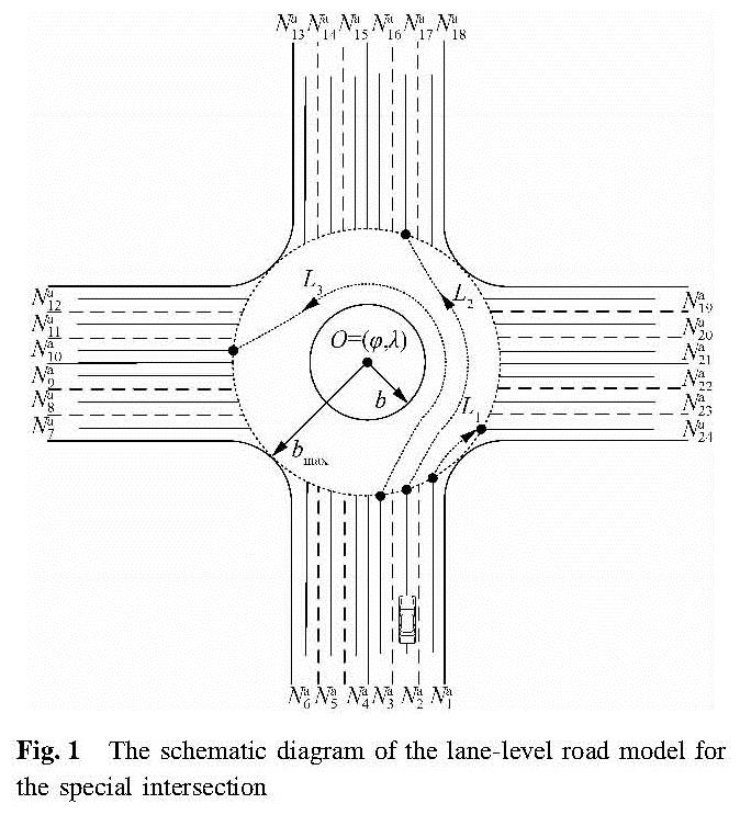
Under various considerations, the lane-level road model for the special intersection is defined as where Q is the set of the basic attributes of the special intersection; V is the set of the virtual lanes inside the intersection.

M=(Q,V)(1)

Fig.1 shows the schematic diagram of the lane-level road model for the special intersection.The set of the basic attributes of the special intersection Q is defined as where N_c is the serial number of the intersection; O is the coordinate of the center point of the intersection; O=(φ,λ), in which φ is the latitude of the center point and λ is the longitude of the center point; b is the radius of the vegetation or artificial landscape area in the middle of the intersection. Specially, it is a general intersection when vegetation or artificial landscape is not included(b=0). b_max is the maximum radius of this intersection. U is the set of actual lanes which are connected to the intersection, U={N^a₁,N^a₂,…,N^a_d}, in which N^a_d is the serial number of the d-th connected actual lane.

Q=(N_c,O,b,b_max,U)(2)

Fig.1 The schematic diagram of the lane-level road model for the special intersection

The set of the virtual lanes inside the intersection V is defined as where L_m is the set of basic attributes of the m-th virtual lane.

V=(L₁,L₂,L₃,…,L_m)(3)

Additionally, L can be further expressed as where N^v is the serial number of the virtual lane inside the intersection; N^a_out and N^a_in are the serial number of the actual departure lane and actual enter lane which are connected to the virtual lane, respectively. G is the set of control points that describe the geometrical structure of the virtual lane, G={(x₁,y₁),(x₂,y₂),…,(x_n,y_n)}, in which x_n,y_n are the latitude and longitude of the n-th control point, respectively. A is the parameter set of the spline curve fitting the virtual lane.

L=(N^v,N^a_out,N^a_in,G,A)(4)

In this paper, we choose the cardinal spline to represent the geometrical structure of the model. The cardinal spline is specified by a series of control points and tension parameters. A gradual optimization algorithm will be introduced in detail in the next section which determines reasonable control points and optimal tension parameters under different traffic situations at the special intersection.

Currently,the spline curve can generally be divided into two categories: approximating spline and interpolating spline. The cardinal spline is a family of interpolating splines^[20-21]. To the best of the authors' knowledge, the cardinal spline has been studied for a long time in the field of the CAD/CAM industry and the cardinal spline representation of the road geometry structure was rarely applied in the field of road modeling in the previous literature.

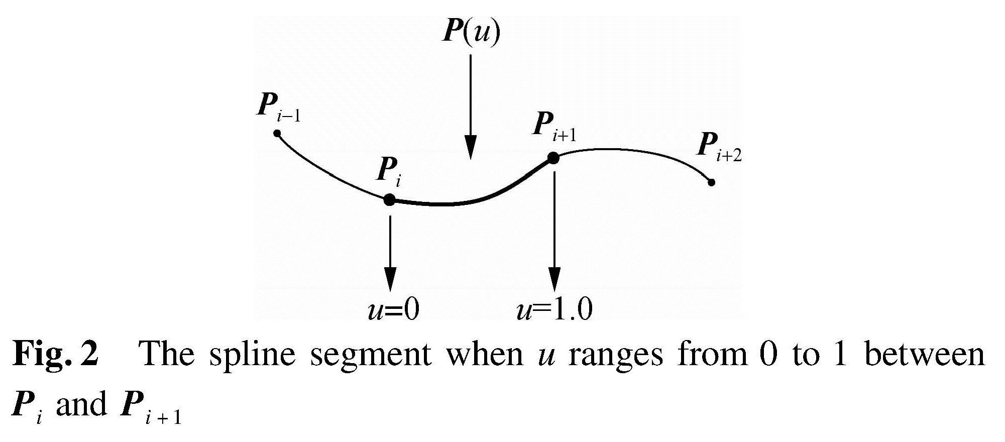
The cardinal spline is specified by a series of control points and tension parameters. A cardinal spline passes smoothly through each control point. It is a sequence of individual piecewise cubic curves joined to form a larger curve, and each cardinal spline segment is defined by four control points P_i-1, P_i, P_i+1, P_i+2, with the curve drawn only from P_i to P_i+1. The tangent vector at each control point P_i is calculated using the previous and next control point on the spline. A single cardinal spline segment can be completely determined by four consecutive control points, in which the middle two control points are the endpoints of the cardinal spline segment and the other two control points are used to calculate the tangents at the endpoints of the cardinal spline segment. Assume that P_i-1, P_i, P_i+1, P_i+2 are four given consecutive control points(each of them has x and y values)and P(u)is a parametric cubic polynomial between control points P_i and P_i+1. Hence, the boundary condition for establishing a single cardinal spline segment using four points P_i-1 to P_i+2 is where P(0)and P(1)are the position vectors of P(u)at the two endpoints of the spline segment between P_i and P_i+1, respectively. u is the parameter of the spline segment and ranges from 0 to 1 between P_i and P_i+1(see Fig.2).

(5)

Fig.2 The spline segment when u ranges from 0 to 1 between Pi and Pi+1

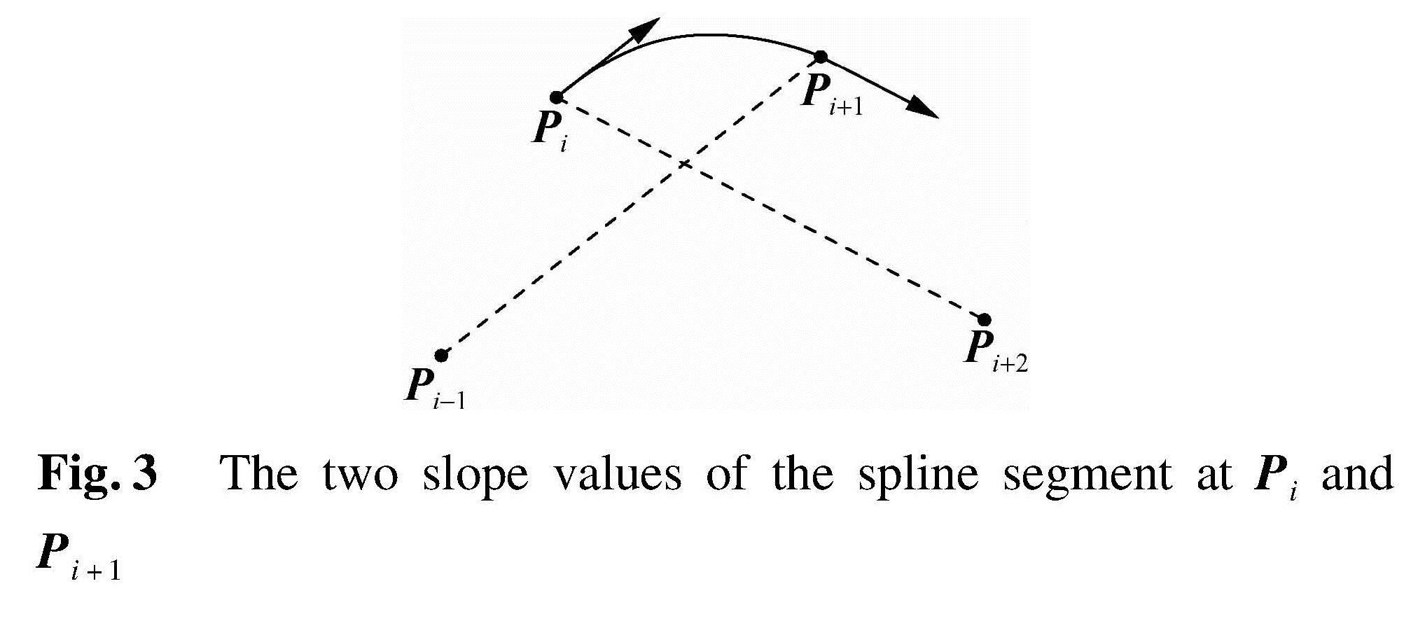
P'(0)and P'(1)are the tangent vectors of P(u)at the two endpoints of the spline segment between P_i and P_i+1, respectively.The two slope values of the spline segment at P_i and P_i+1 are proportional to chord P_i-1P_i+1^→ and P_iP_i+2^→, respectively(see Fig.3).

Fig.3 The two slope values of the spline segment at Pi and Pi+1

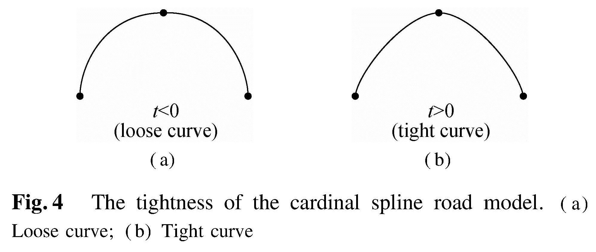
The parameter t is a tension parameter which affects the tightness of the cardinal spline. When t>0, the cardinal spline curve is called a tight curve. When t<0, the cardinal spline curve is called a loose curve(see Fig.4). When t=0, the cardinal spline curve is called a Catmull Rom spline curve.

Fig.4 The tightness of the cardinal spline road model.(a)Loose curve;(b)Tight curve

The four equations in the solution(5)are converted into a matrix form as follows:

(6)

where the cardinal matrix is as follows:

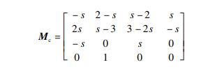(7)

where s=1-t/2.

In Eq.(6), the matrix equation is expanded into a polynomial form:

P(u)=P_i-1(-su³+2su²-su)+P_i[(2-s)u³+(s-3)u²+1]+P_i+1[(s-2)u³+(3-2s)u²+su]+P_i+2(su³-su²)(8)

Now, we can decompose Eq.(8)into the components of the x and y directions on the two-dimensional plane, and obtain the following expression of the cubic polynomial of the spline segment between control points P_i and P_i+1 in the x and y directions:

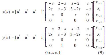
Then, after the expansion of Eq.(9), the cardinal spline segment between control points P_i and P_i+1 is given as

x(u)=Aⁱ₀+Aⁱ₁u+Aⁱ₂u²+Aⁱ₃u³

y(u)=Bⁱ₀+Bⁱ₁u+Bⁱ₂u²+Bⁱ₃u³

0≤u≤1(10)

where

Aⁱ₀=x_i

Aⁱ₁=-sx_i-1+sx_i+1

Aⁱ₂=2sx_i-1+(s-3)x_i+(3-2s)x_i+1-sx_i+2

Aⁱ₃=-sx_i-1+(2-s)x_i+(s-2)x_i+1+sx_i+2

Bⁱ₀=y_i

Bⁱ₁=-sy_i-1+sy_i+1

Bⁱ₂=2sy_i-1+(s-3)y_i+(3-2s)y_i+1-sy_i+2

Bⁱ₃=-sy_i-1+(2-s)y_i+(s-2)y_i+1+sy_i+2

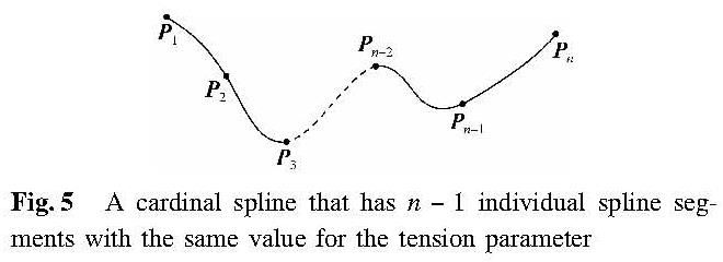
Thus, it can be seen that each cardinal spline segment is specified by the four given consecutive control points and a tension parameter which is determined according to the control requirements and accuracy requirements of the actual application scenarios. Generally, we suppose that P₁ and P_n are the starting point and the ending point of a given series of control points, respectively. Then, the spline segment drawn from P₁ to P₂ is specified by P₁, P₁, P₂, P₃ and the spline segment drawn from P_n-1 to P_n is specified by P_n-2, P_n-1, P_n, P_n similarly. Fig.5 shows a cardinal spline that has n-1 individual spline segments with the same value for the tension parameter.

Fig.5 A cardinal spline that has n-1 individual spline segments with the same value for the tension parameter

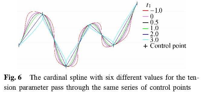
The cardinal spline with different values for the tension parameter will produce different curves through a given series of control points. As shown in Fig.6, the cardinal spline with six different values for the tension parameter passes through the same series of control points. The tension parameter t is shown in Fig.6 for different values.

Fig.6 The cardinal spline with six different values for the tension parameter pass through the same series of control points

Note that the cardinal splines in Fig.6 share the same tangent line at the starting point which is the line drawn from the starting point to the next point along the curve. Likewise, the shared tangent at the ending point is the line drawn from the ending point to the previous point on the curve. The tangent line at other points is parallel to the line drawn from the previous point to the next point along the curve.

An optimization algorithm of the intersection model is proposed to determine reasonable control points and optimal tension parameters under different traffic situations at the special intersection. We select reasonable control points for the cardinal spline according to different traffic situations, which can improve the data storage efficiency of the intersection model. Additionally, the value of the tension parameter for each individual cardinal spline segment will be adjusted to satisfy the desired accuracy until the error between the roadway data points and the cardinal spline reaches an acceptable range, which can better approximate the real vehicle trajectory at the special intersection. In this paper, a probe vehicle equipped with a single-enclosure GPS+INS positioning system measures the roadway data points of the special intersection and the acquired data will be processed manually to remove the outliers.

In general circumstances, traffic situations at the special intersection can be divided into the following three categories: turn right, turn left and go straight. For these three different traffic situations, we separately select different points as the control points of the cardinal spline which can represent the geometrical structure of the intersection model.

Therefore, G can be further expressed as

(11)

where E is the endpoint of the lane which enters the intersection; E' is the control point of 10 m apart from point E on the enter lane; D is the starting point of the lane which exits the intersection; D' is the control point of 10 m apart from point D on the departure lane.

Then, we use the above series of points as the control points of the cardinal spline and gradually adjust the value of the tension parameter for each individual cardinal spline segment until the error between the given roadway data points and the cardinal spline meets an acceptable range. This can better approximate the real right-turn trajectory of the vehicle at the intersection.

Next, the selection process of the control points under different traffic situations at the intersection is described in detail.

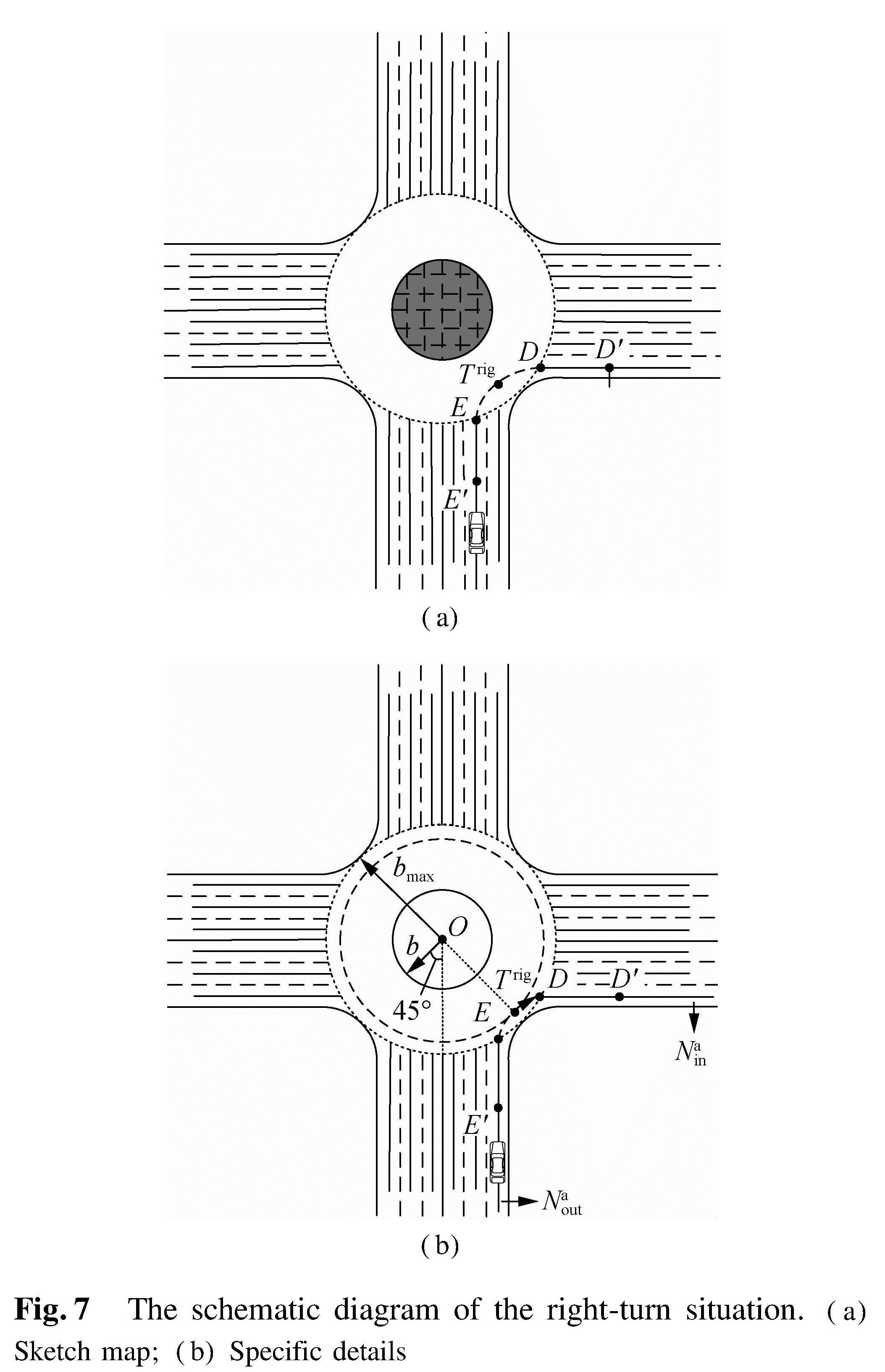
For the right-turn situation, G can be specifically expressed as

G={E',E,T ^rig,D,D'}(12)

where T ^rig is a special control point selected for the right-turn situation, and it is the point at which a straight line with a 45° angle to the centerline is intersected by a circle with point O as a center point and a radius of(b+10)m. As shown in Fig.7(a), G={E',E,T ^rig,D,D'} is a set of control points arranged in order by the right-turn trajectory of the vehicle at the special intersection.The specific details are shown in Fig.7(b).

Fig.7 The schematic diagram of the right-turn situation.(a)Sketch map;(b)Specific details

For the go-straight situation, G can be specifically expressed as

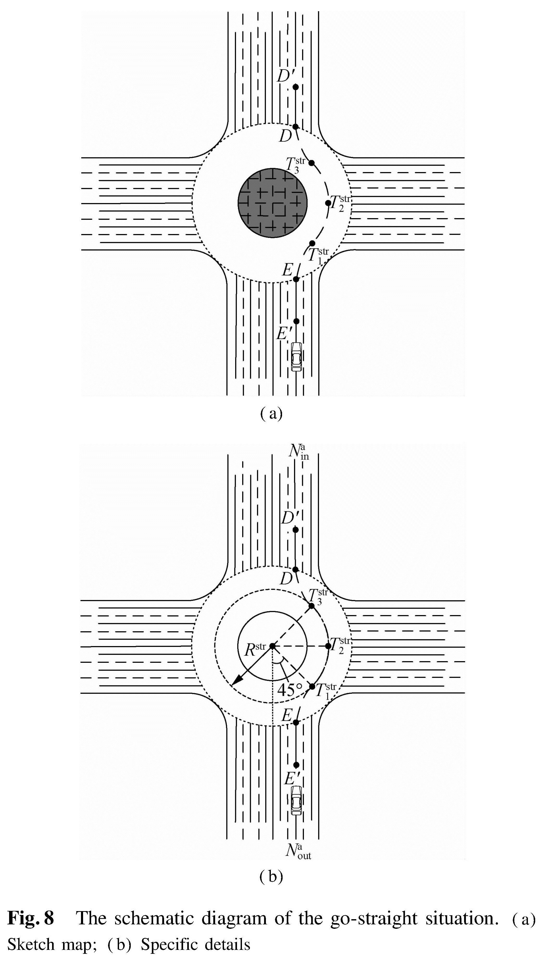
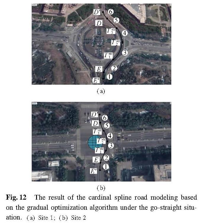
G={E',E,T ^str₁,T ^str₂,T ^str₃,D,D'}(13)

where T ^str₁, T ^str₂, T ^str₃ are the special control points selected for the go-straight situation; T ^str₁ is the point at which a straight line with a 45° angle to the centerline is intersected by a circle with point O as a center point and a radius of(b+6)m; T^str₂ is the point at which a straight line with a 90° angle to the centerline is intersected by this circle; T^str₃ is the point at which a straight line with a 135° angle to the centerline is intersected by this circle.

As shown in Fig.8(a), G={E',E,T ^str₁,T ^str₂,T ^str₃,D,D'} is a set of control points arranged in order by the go-straight trajectory of the vehicle at the special intersection. The specific details are as shown in Fig.8(b).

Fig.8 The schematic diagram of the go-straight situation.(a)Sketch map;(b)Specific details

For the left-turn situation, G can be specifically expressed as

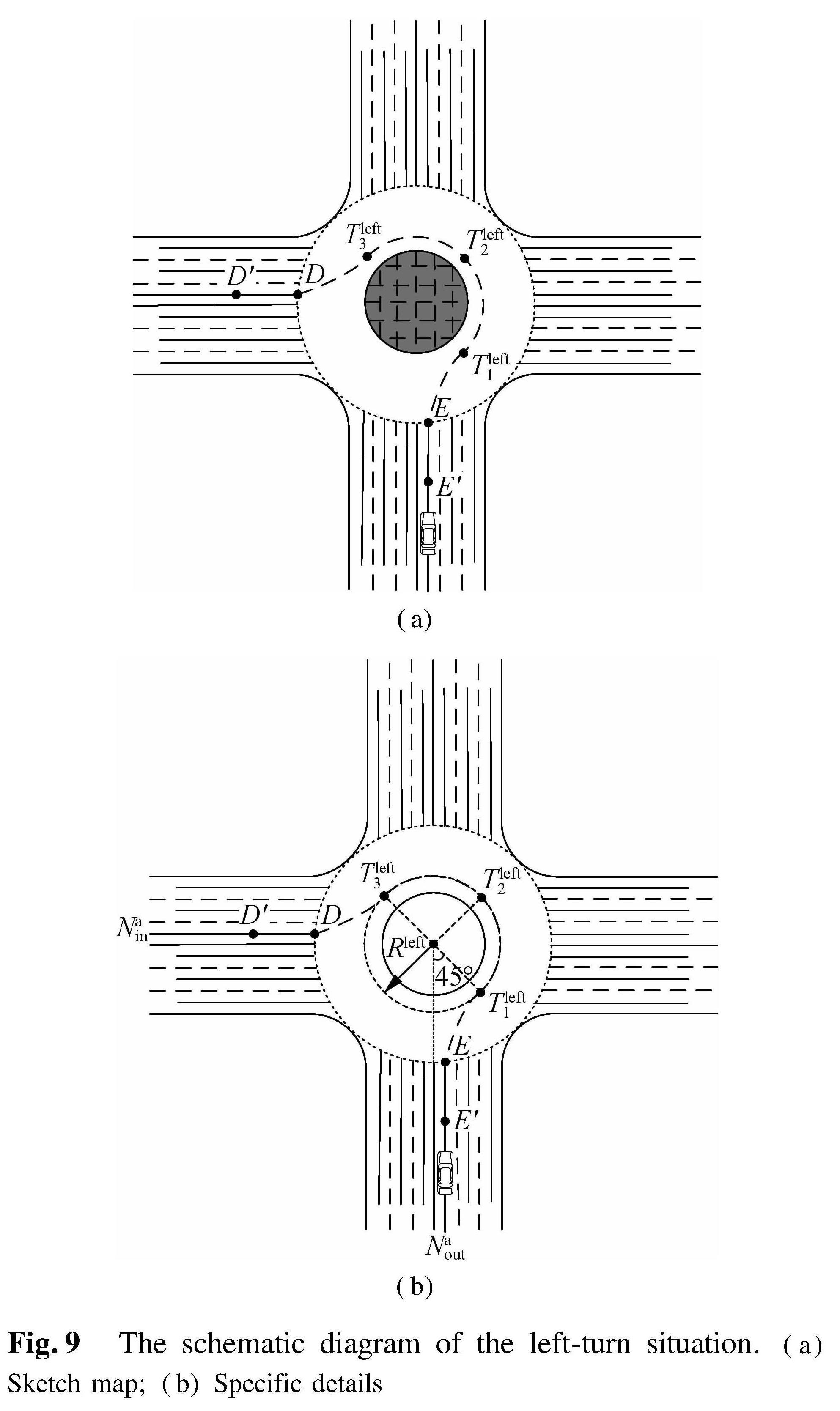
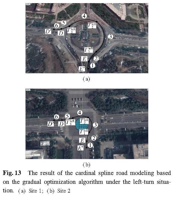
G={E',E,T ^left₁,T ^left₂,T ^left₃,D,D'}(14)

where T ^left₁, T ^left₂, T ^left₃ are the special control points selected for the left-turn situation; T^left₁ is the point at which a straight line with a 45° angle to the centerline is intersected by a circle with point O as a center point and a radius of(b+2)m; T^left₂ is the point at which a straight line with a 135° angle to the centerline is intersected by this circle; T^left₃ is the point at which a straight line with a 225° angle to the centerline is intersected by this circle.As shown in Fig.9(a), G={E',E,T^left₁,T^left₂,T^left₃,D,D'} is a set of control points arranged in order by the left-turn trajectory of the vehicle at the special intersection.The specific details are as shown in Fig.9(b).

Fig.9 The schematic diagram of the left-turn situation.(a)Sketch map;(b)Specific details

In the previous step, reasonable data points were selected as the control points of the cardinal spline curve. The selection of the optimal threshold value needs to take the efficiency and reliability of the road model into consideration. Therefore, the tension parameter is first set to be -1 for each cardinal spline segment determined by a series of control points obtained in the previous step. Then, the tension parameters of each cardinal spline are adjusted step by step independently by comparing the error between the cardinal spline and reference. Each adjustment increases by 0.1 until the cardinal spline has the smallest error to the reference.Generally speaking, the adjustment range of tension parameters is between -1 and 2.

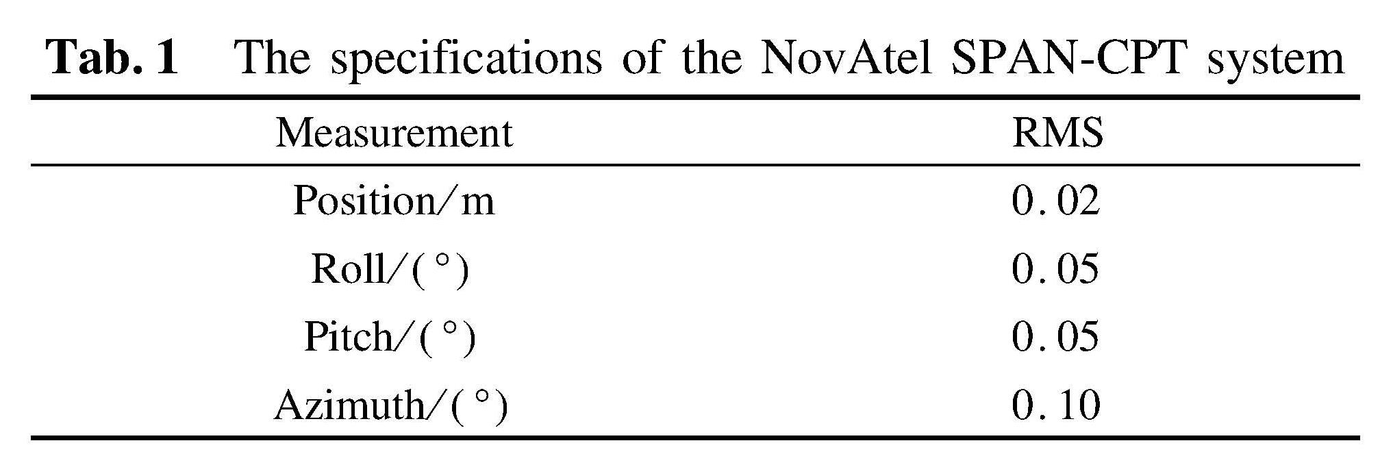
To evaluate the performance of the proposed lane-level road model for the special intersection, experiments were carried out on a Chery TIGGO5 SUV vehicle. The raw roadway data points of the special intersection were collected using the probe vehicle equipped with a GPS+INS vehicle positioning system(NovAtel SPAN-CPT system). The NovAtel SPAN-CPT system is an accurate and reliable GPS+INS vehicle positioning system, which can provide accurate and reliable positioning information via post-processing even under adverse environments. The specifications of the NovAtel SPAN-CPT system are summarized in Tab.1. In this paper, the probe vehicle was driven at a stationary driving speed of 30 to 50 km/h along the centerline of the lane.

Tab.1 The specifications of the NovAtel SPAN-CPT system

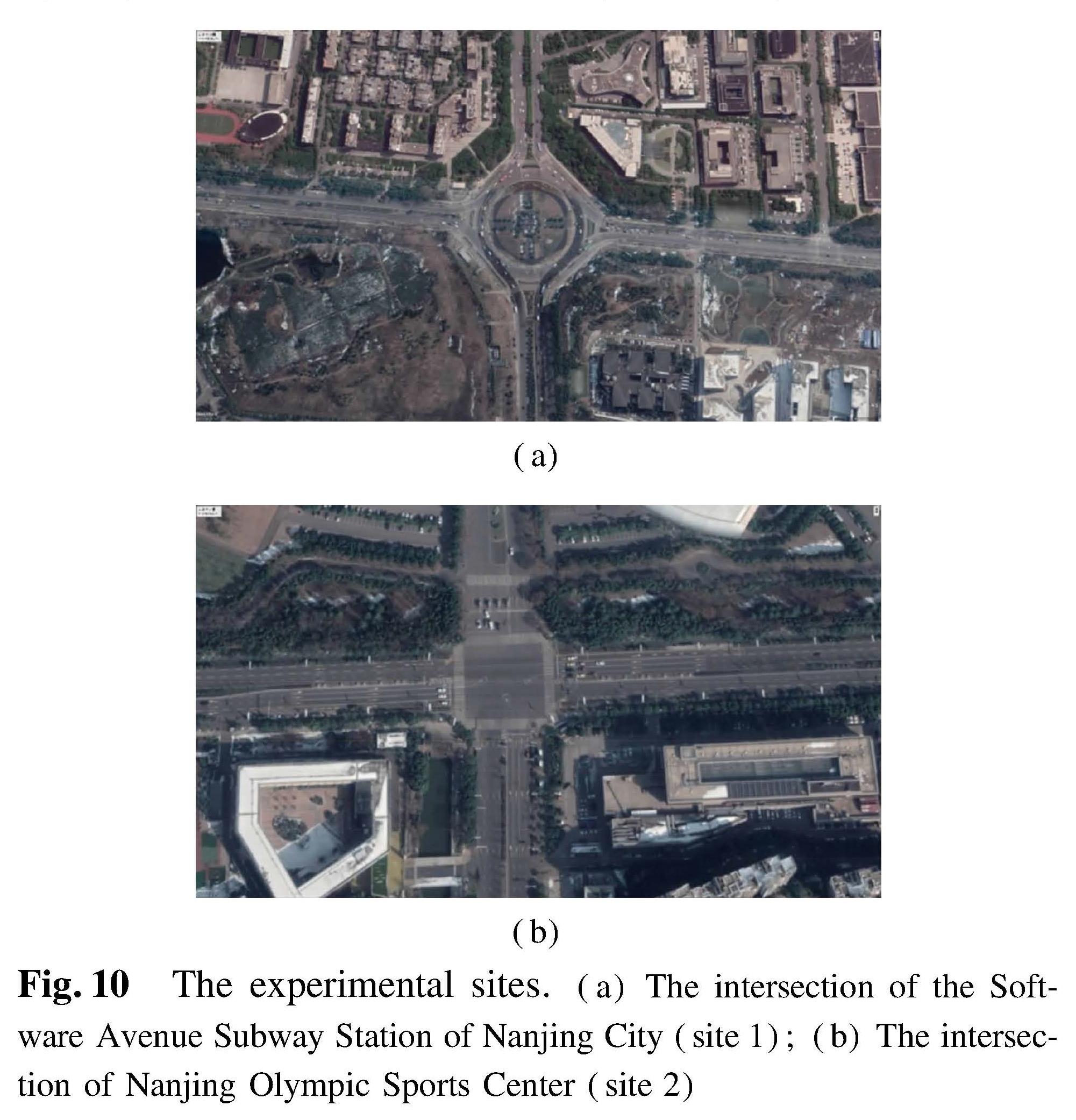
The experiments were executed at the intersections of the Software Avenue Subway Station of Nanjing City and Nanjing Olympic Sports Center. These intersections are typical special intersections which are covered by vegetation in their central regions. Fig.10 shows the

Fig.10 The experimental sites.(a)The intersection of the Software Avenue Subway Station of Nanjing City(site 1);(b)The intersection of Nanjing Olympic Sports Center(site 2)

experimental sites. Figs.11 to 13 show the trajectories of the probe vehicle at the intersections under three traffic situations(right-turn, go-straight, left-turn).

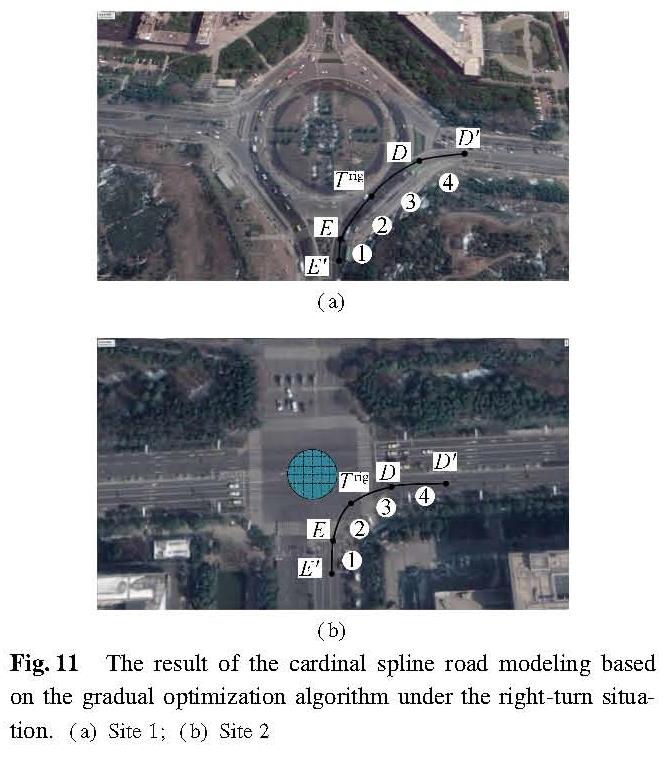
Fig.11 The result of the cardinal spline road modeling based on the gradual optimization algorithm under the right-turn situation.(a)Site 1;(b)Site 2

Fig.12 The result of the cardinal spline road modeling based on the gradual optimization algorithm under the go-straight situation.(a)Site 1;(b)Site 2

We use the gradual optimization algorithm mentioned above to determine reasonable control points and optimal tension parameters for the cardinal spline at this intersection under three traffic situations.Reasonable control points for the cardinal spline can improve the data storage efficiency of the model. Additionally, the value of the tension parameter for each individual cardinal spline segment will be gradually adjusted to satisfy a desired accuracy until the error between the roadway data points and the cardinal spline meets an acceptable range. Fig.11 shows the result of the cardinal spline road modeling based on the gradual optimization algorithm under the right-turn situation. Fig.12 shows the result of the cardinal spline road modeling based on the gradual optimization algorithm under the go-straight situation. Fig.13 shows the result of the cardinal spline road modeling based on the gradual optimization algorithm under the left-turn situation.

Fig.13 The result of the cardinal spline road modeling based on the gradual optimization algorithm under the left-turn situation.(a)Site 1;(b)Site 2

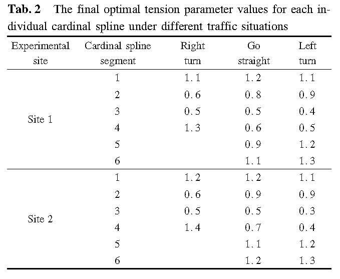
As can be seen from Figs.11 to 13, there are five control points and four individual cardinal spline segments under the right-turn situation, seven control points and six individual cardinal spline segments under the go-straight situation, seven control points and six individual cardinal spline segments under the left-turn situation. The final optimal values of the tension parameter for each individual cardinal spline under different traffic situations are shown in Tab.2.

Meanwhile,the final right-turn virtual lane with cardinal spline fitting achieves the global accuracy of 1.05 m at Site 1 and 1.24 m at Site 2 by using five control points.The final go-straight virtual lane with cardinal spline fitting achieves the global accuracy of 1.24 m at Site 1 and 1.31 m at Site 2 by using seven control points. The final left-turn virtual lane with cardinal spline fitting achieves the global accuracy of 1.35 m at Site 1 and 1.36 m at Site 2 by using the seven control points.

Tab.2 The final optimal tension parameter values for each individual cardinal spline under different traffic situations

From the experimental results above, we can see that the cardinal spline road modeling based on the gradual optimization algorithm uses a small number of control points to meet a desired lane-level accuracy under three traffic situations. It is clear that the topological structure of the model can effectively describe the connectivity, turn restrictions and other attributes of this kind of intersection in the real world, and the geometrical structure of the model can effectively describe the virtual lanes of the internal part of this kind of intersection. In general, this method can balance the efficiency and reliability requirements of the special intersection.

1)A lane-level road model is proposed for the special intersections which are covered by vegetation or artificial landscape in their central regions.

2)The main contribution of this paper is to adopt the cardinal spline road modeling based on the optimization algorithm to represent the geometrical structure of the special intersections, which can better approximate the real vehicle trajectory at the intersections. Also, a gradual optimization algorithm is presented to determine reasonable control points and optimal tension parameters for the cardinal spline under different traffic situations at the special intersections.

3)The experiments on two different sites are conducted to demonstrate that the lane-level special intersection model proposed in this paper occupies less data storage and achieves considerable accuracy.