Empirical mode decomposition (EMD) is a signal processing algorithm proposed by Huang et al.[1-2] in 1998. It has many significant advantages for processing nonlinear and non-stationary signals and has achieved huge progress and achievements in various fields such as radio signals and medical EEG signals[3-4]. As the theory of the algorithm has not been strictly proved, there are still some problems in the process of data decomposition, one of which is the end effect. In the decomposition process, the upper and lower envelopes are obtained by interpolating signal extremes to form a cubic spline curve, but the endpoints of signal may not be extremes, which diverges envelopes at the end of signal. The presence of divergence will seriously affect the accuracy and effectiveness of the decomposition results, especially when using EMD for time series analysis and fault diagnosis. Scholars have studied several effective methods to constrain the end effect. On the one hand, one kind of method that uses other splines to fit envelops has an inhibitory effect on the end effect, and it is rarely used since its practical performance is worse than using cubic splines[5]. On the other hand, signal extension methods such as mirror extension, waveform matching extension, polynomial fitting prediction, neural network prediction and other methods are quite effective for constraining the end effect[6]. Wang et al.[7] proposed a method combining mirror extension and SVM to constrain end effect. Hao et al.[8] proposed a new method of adding windows function to SVM extension signals to constrain the end effect. Furthermore, the extension algorithm based on waveform matching extends the similar waveform at the end of the signal, and it takes into account the change trend inside and at the end of the signal. It has advantages unmatched by other methods and has become one of the important ways to constrain the end effect of EMD. The traditional waveform matching extension can play an effective role in constraining the end effect, and its improved methods are proposed in the follow-up studies which optimize the algorithm and its accuracy for the end effect problem. Shao et al.[9] applied the waveform matching method based on the distance function to the EMD endpoint extension and achieved good results. Su et al.[10] proposed the gray mean prediction model to extend the original data to reduce the end effect; Xu et al.[11] symbolized the signal local extreme value sequence to extend according to feature matching and reduced the impact of the end effect. However, these algorithms have some shortcomings that largely depend on the accuracy and efficiency of the initial data matching. If there is some deviation between original data, the extended waveform will not match the actual situation. Therefore, this paper proposes an end effect suppression method based on a sequential similarity matching and adaptive filter, and processes the simulation signal and the experimental signal by using this method. The results show that this method can effectively prevent the occurrence of the end effect.
1 EMD and the End Effect
1.1 EMD
EMD is representative in the adaptive time-frequency analysis method. Its main principle is to separate the intrinsic mode function (IMF) from the complex signal. These IMFs need to satisfy the following two conditions: In the whole data set, the number of extreme is equal and the number of zero crossings must either be equal to or differ at most by one; at any point, the mean value of the envelope defined by the local maxima and envelope defined by the local minima is zero[1]. The flow chart is shown in Fig.1.
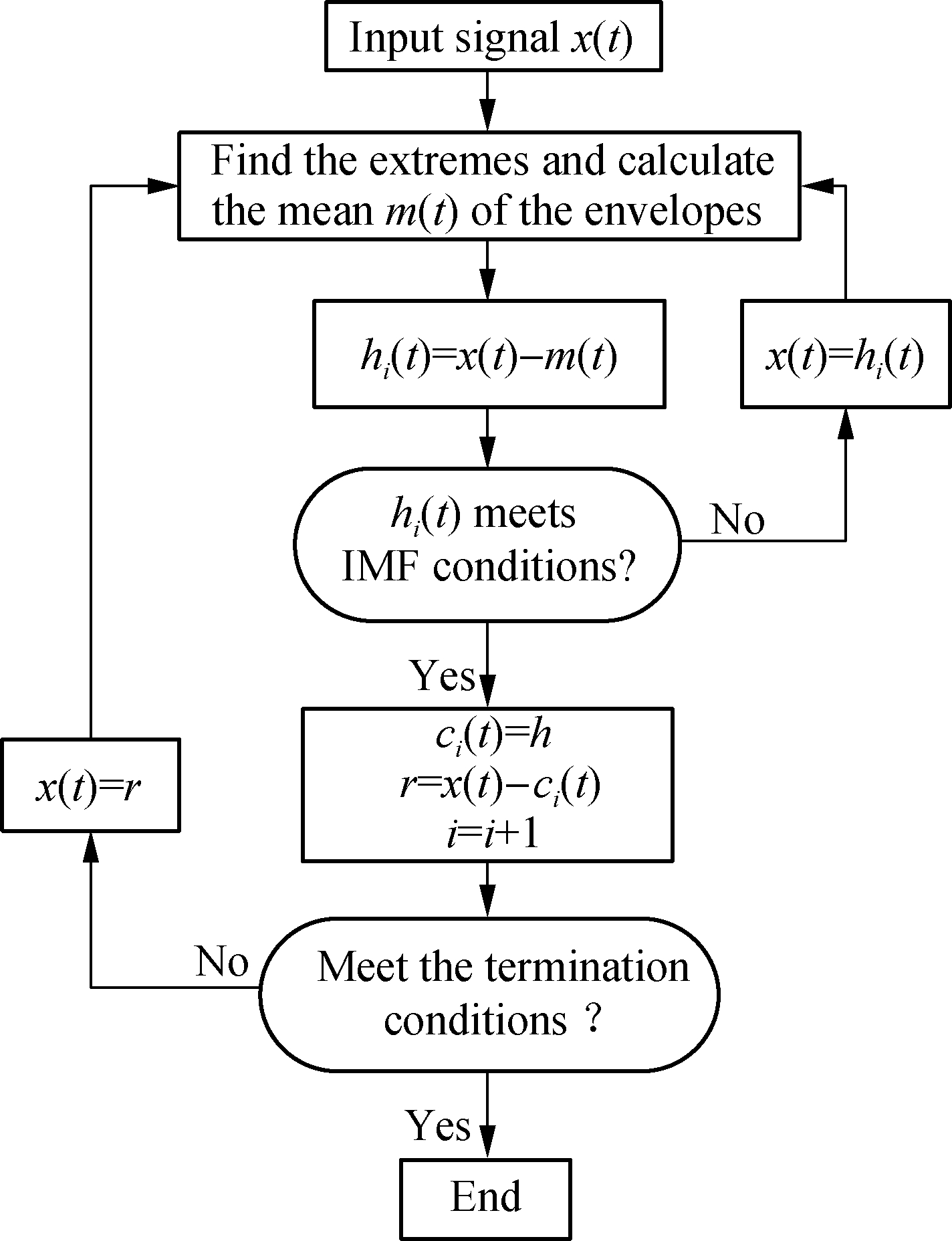
Fig.1 EMD flow chart
The specific decomposition process is as follows:
1) All extremes of the initial signal x(t) are found, and cubic splines are used to fit the maxima and construct the upper envelope. Similarly, the minima is used to construct the lower envelope, and the mean m(t) of two envelopes is calculated. Then, the IMF h1(t) can be calculated by
h1(t)=x(t)-m(t)
(1)
2) Check whether above IMF conditions are satisfied. If not, let m(t)=h1(t) and repeat step 1) k times. On the contrary, an IMF component representing the highest frequency of the initial signal is obtained which is recorded as c1(t).
c1(t)=h1k(t)=h1(k-1)(t)-m1k(t)
(2)
3) x(t) is separated from c1(t) and the remainder r1(t) is obtained.
r1(t)=x(t)-c1(t)
(3)
4) The steps above are repeated n times until rn(t) meets the given termination condition. The decomposition is completed, and n IMFs and a remainder are obtained. The initial signal can be expressed as
(4)
where rn(t) is the remainder representing the average trend of the signal; ci(t) contains IMF components from high to low frequencies.
1.2 End effect
When the signal is decomposed by an EMD, it is necessary to interpolate the extreme with a cubic spline curve. Since the two endpoints of signal cannot be determined to be extremes, it will make the envelope swing larger near the endpoints. With the decomposition in progress, errors will propagate and accumulate inward from the endpoints, which eventually lead to an inaccurate result[12]. This is the end effect of EMD.
Take the simulation signal as an example to illustrate the end effect. The simulation signal is
(5)
Fig.2 shows the curve obtained by using cubic splines directly to fit the extreme of the simulation signal. Since it is impossible to determine whether the extreme is at the end of the signal, large oscillation occurs at both ends of the signal during fitting and results in serious distortions of the decomposition signal. Therefore, it is necessary to eliminate or reduce the end effect by extending the end point appropriately.
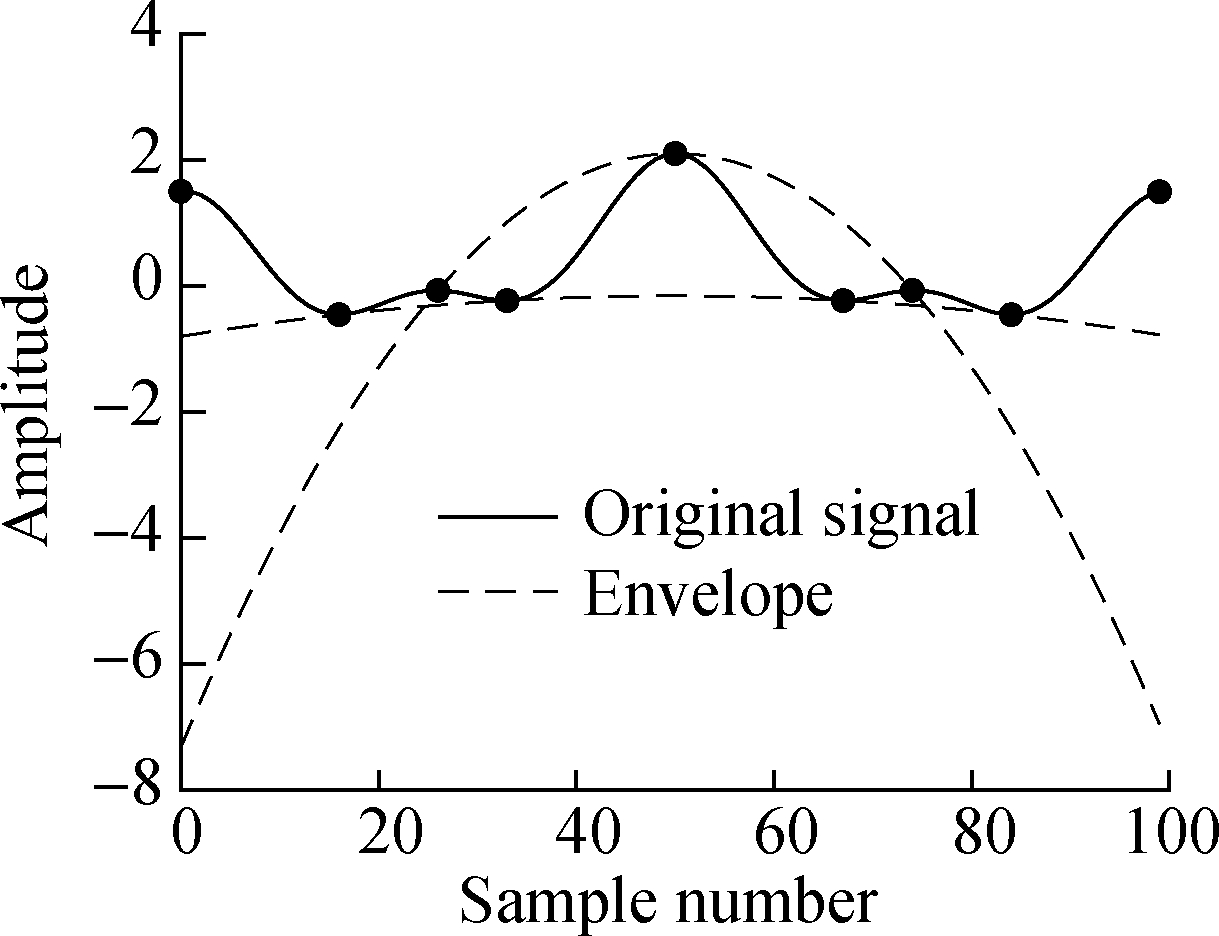
Fig.2 The end effect of EMD
2 Adaptive Similar Waveform Matching Exten-sion
2.1 Traditional waveform matching extension method
The waveform matching extension method is one of the end effect suppression methods, and its key aim is that the change trend at the signal end is also reflected internally, especially for signals with strong regularity. Its specific process mainly includes two parts: 1) Find the waveform inside the signal that has the same trend as the end signal; 2) Translate the best matching waveform to the signal end and extend it. Fig.3 shows the distance-based waveform matching process, and the matching distance of the two wavelets is
(6)
where s1(i) and sj(i) are the values of the i-th sampling point of the initial and matched wavelet, respectively; and N is the data length of the wavelet. A waveform including at least two extremes in front of wavelet S1 that has minimum matching distance is taken and is translated to the signal end to achieve extension.
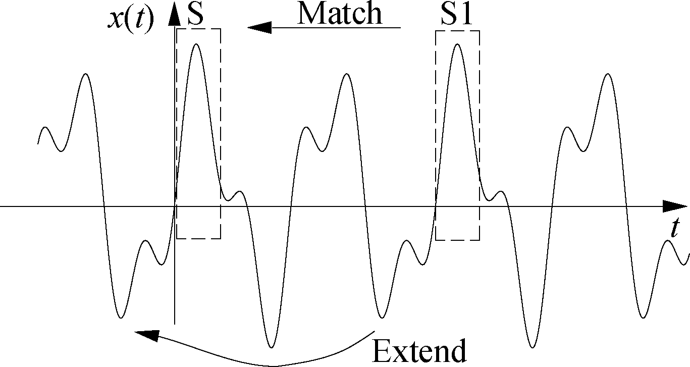
Fig.3 Distance-based waveform matching process
The traditional waveform matching extension can suppress the end effect, but there are certain shortcomings as follows:
1) Intercepting meaningless wavelet
As shown in Fig.4, when the wavelets are intercepted at equal lengths and the length of the initial waveform S is not selected properly, meaningless wavelets appear. These wavelets cannot match the initial waveform, in which S1 contains two minimum points and S2 contains two maximum points. Meaningless wavelets waste matching calculation time, and make the matching algorithm inefficient and even lose actual meaning.
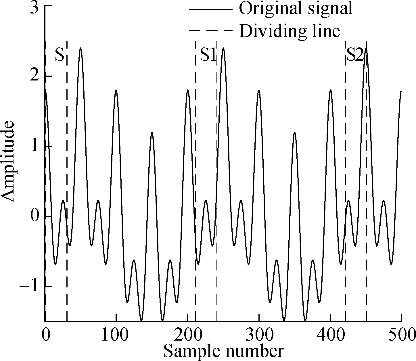
Fig.4 Meaningless wavelet interception
2) Matching error caused by discrete data
Since the computer can only process discrete data, a matching error will inevitably occur when the sampling frequency is not a common multiple of all frequency components of the original signal. It also affects the matching accuracy to some extent. Take the simulation signal as an example as follows:
x(t)=cos(100πt)+sin(70πt)
(7)
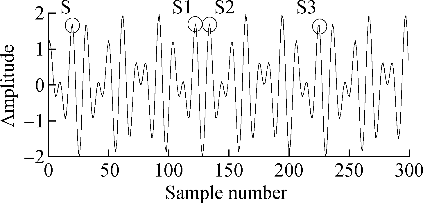
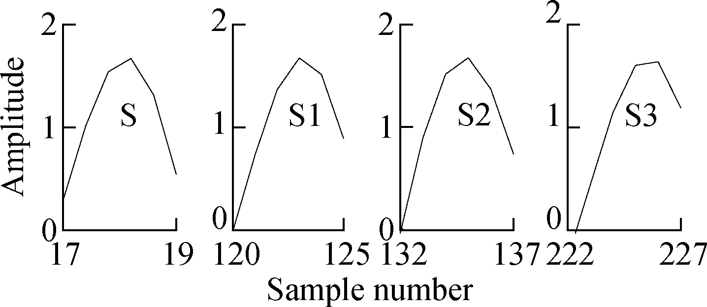
The sampling frequency is 512 Hz, and the sampling number is 300. The image is shown in Fig.5 and the matching distance is shown in Tab.1. From the detailed window and table, it can be seen that S1 and S3 wavelets should be matched, but S2 wavelet is finally selected due to the difference of discrete data in the matching distance. This is a matching error. In addition, the difference may cause more inaccurate matching errors for random waveform with strong noise.
(a)
(b)
Fig.5 Matching errors caused by discrete data.(a) Simulation signal; (b) Local waveform
Tab.1 Waveform matching distance
S1S2S30.354 10.162 41.322 3
2.2 Waveform matching extension based on sequential similarity detection and adaptive filter
Sequential analysis comes from mathematical statistics. Its purpose is to use the samples to make statistical inferences[13-14]. The method does not specify sample number in advance, but takes a small sample and decides whether to continue sampling, so it can reduce the sample number effectively.
The sequential similarity detection algorithm (SSDA) is widely used in signal matching and other fields due to its low computational complexity and high accuracy. The threshold is generally adjusted until the best matching wavelet is selected during matching the signal. The best matching wavelet does not necessarily meet expansion requirements according to the previous descriptions, so this paper selects multiple wavelets that meet the conditions by adjusting the threshold to extend waveform. The selection and adjustment of the cut-off threshold plays a very important role in wavelet selection. The usual cut-off threshold uses the matching distance mentioned above and the amplitude of the matched wavelet is not considered, so it is difficult to intuitively reflect the matching accuracy of the matching wave, which is not conducive to threshold selection. Therefore, in this paper, the matching distance is divided by the square of the initial wavelet extreme difference to standardize the matching distance. In addition, the variance of the difference between matching wavelets is calculated to prevent sudden changes in the waveform. The method of adjusting threshold by the folding mode can speed up the matching rate.
The processed multiple wavelets are sorted in time series, and then the adaptive filter method[15-16] is used to extend the endpoints. The basic prediction formula is
(8)
where ![]() is the predicted value of the (t+1)-th wavelet; wi is the observed weight value of the (t-i+1)-th wavelet; yt-i+1 is the observed value of the (t-i+1)-th wave; N is the number of weights. The formula for adjusting the weight is
is the predicted value of the (t+1)-th wavelet; wi is the observed weight value of the (t-i+1)-th wavelet; yt-i+1 is the observed value of the (t-i+1)-th wave; N is the number of weights. The formula for adjusting the weight is
(9)
where i=1,2,…,N; t=N,N+1,…,n; n is the number of sequence data; wi is the i-th weight before adjustment; w′i is the i-th weight after adjustment; k is the learning constant; ei+1 is the prediction error of the (t+1)-th wavelet. k is generally set to be 1/N to indicate the rate of weight adjustment.
The advantages of sequential similarity detection and adaptive filtering are effectively combined to ensure the accuracy and speed of the new matching extension algorithm that can complete the endpoint extension successfully.
The specific steps are as follows:
1) The original wavelet at the end point is determined as X1. The length of this wavelet is K=s+v, where s is the length of the wavelet containing the first maxima and minima, and initially v=1. The ordinates corresponding to the maximum and minimum of X1 are denoted as M and m, respectively, and the slope of the straight line constructed by these two points is denoted as ki.
2) The signal X1 is divided into p segments according to the length of K, and the slopes constructed by their extreme are recorded as ki, i=1,2,…,p, respectively. If |1-ki/k1|≤0.5, the wavelet is recorded in the matching wavelet library Y.
3) The initial cut-off threshold is set to be T1.
4) The accumulative matching error is calculated by ![]() i=1,2,…,K for each wavelet in the matching wavelet library Y. When the cumulative value P is greater than the initial cut-off threshold, this wavelet is discarded to reduce calculation. If P is less than or equal to the initial threshold and the variance is small, this wavelet is a seed wavelet and its position in the entire wave is recorded. All wavelets in library Y are traversed, N seed wavelets are selected.
i=1,2,…,K for each wavelet in the matching wavelet library Y. When the cumulative value P is greater than the initial cut-off threshold, this wavelet is discarded to reduce calculation. If P is less than or equal to the initial threshold and the variance is small, this wavelet is a seed wavelet and its position in the entire wave is recorded. All wavelets in library Y are traversed, N seed wavelets are selected.
5) If the number of seed wavelets, N<1 selected in the above steps, make T2=2T1 and repeat step 4) until several seed wavelets are selected.
6) Make v=1,2,…,n, n is taken as the length of next wave containing two extremes after X1 according to the actual situation. Repeat steps 1) to 5) and take the group of wavelets with the largest number N as the final seed wavelet group.
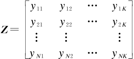
7) If N is less than the set number of weights, the wavelet with the smallest error is translated in the wavelet group for extension. On the contrary, take q sampling points of each wavelet front of the seed wavelet group as the extension wave, arrange the extended wavelet groups in chronological order as
(10)
where yNK is the ordinate value of the K-th sampling point of the N-th seed wavelet.
Each column of Z is predicted to obtain an extended waveform with the adaptive filter method.
The flow chart of the proposed method in this paper is shown in Fig.6.
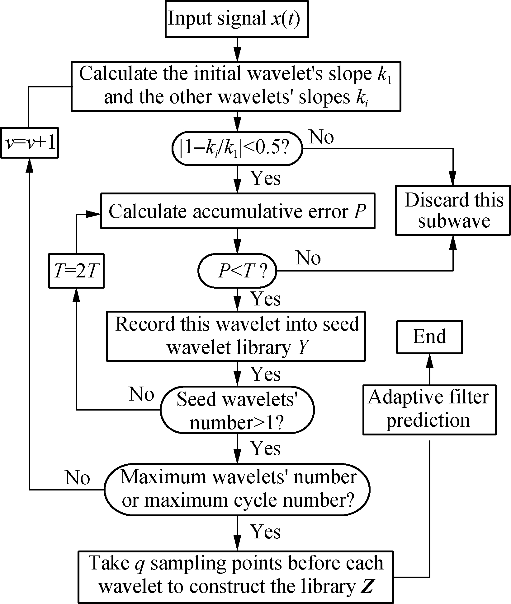
Fig.6 Flow chart of the proposed method
3 Simulation Signal Analysis
In order to verify the effectiveness of the method, this paper uses EMD to analyze the nonlinear and non-stationary simulation signal. This signal simulates the superposition state of the variable frequency amplitude modulation signal and the stable periodic signal, and a discontinuous signal is added to make it a non-stationary signal. The signal expression is

(11)
where the sampling frequency is 3 kHz, and the sampling number is 1 500. The components of signal and the composite signal are shown in Fig.7.

(a)

(b)

(c)

(d)
Fig.7 Original signal and composition. (a) Composite signal; (b) Amplitude modulation signal; (c) Periodic signal; (d) Discontinuous signal
Fig.8 shows each IMF and remainder obtained by direct EMD decomposition of the original signal. The figure shows that if the end effect is not processed, there is some serious deviation at the endpoint and even a false inherent component.
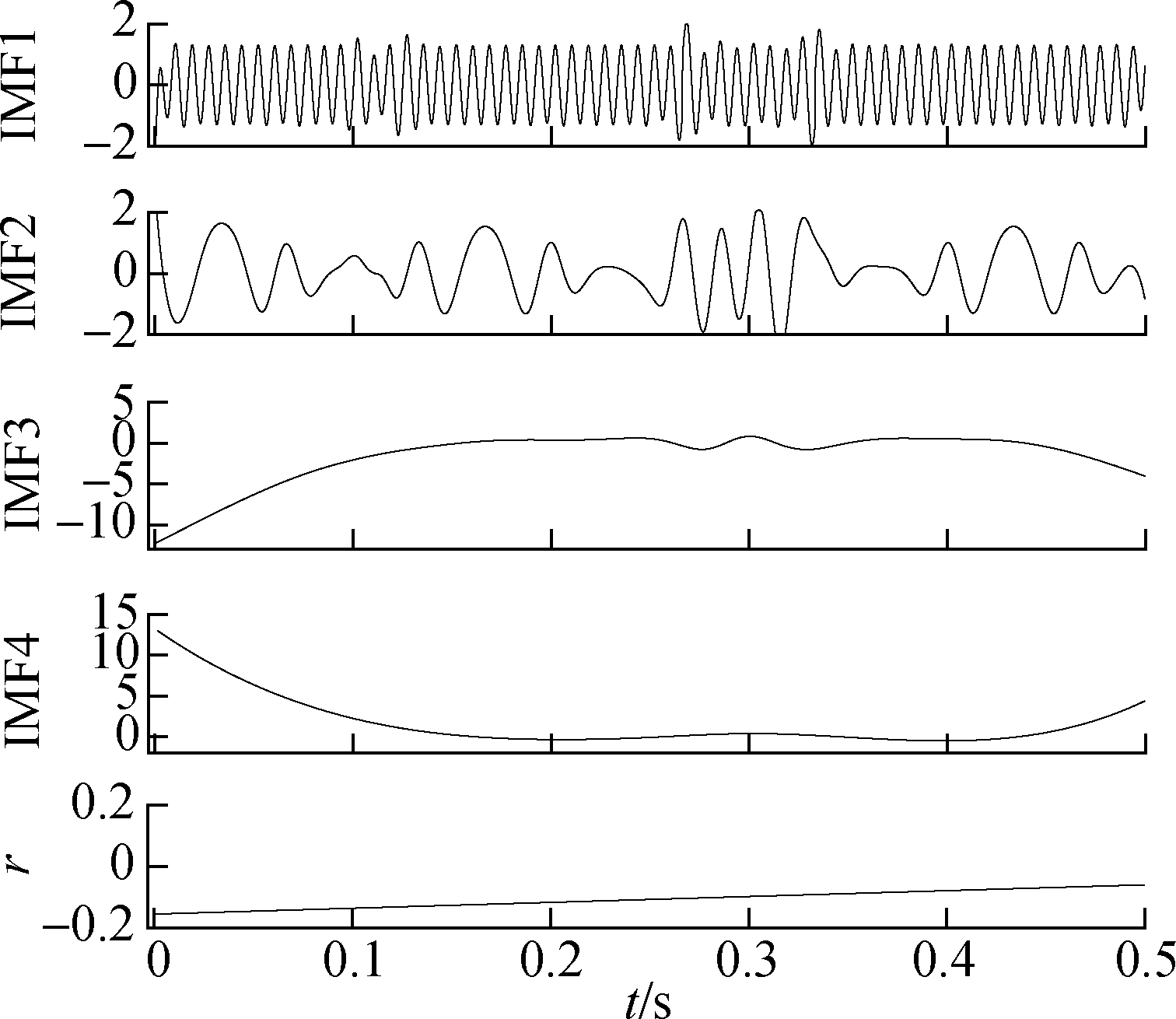
Fig.8 EMD results of original signal
The results of EMD and the Hilbert spectrum of the extended signal by the proposed method are shown in Fig.9 and Fig.10. According to Fig.9, there is no discontinuous signal in the decomposition result due to the modal aliasing effect, and it is mixed into other IMF components. This paper only focuses on the end effect. There is no obvious deviation at the endpoint of each IMF component, and a pseudo component is reduced at the same time. It can be seen from Fig.10 that the frequency at the end point after processing is clearer. Therefore, it indicates that the method in this paper has good suppression for the EMD end effect and is helpful for the subsequent fault diagnosis process.
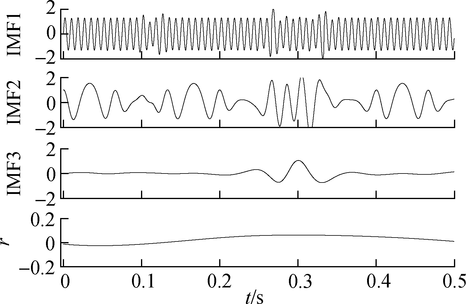
Fig.9 EMD results after extension
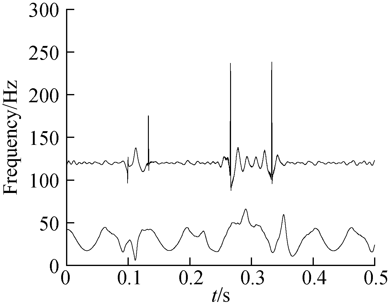
Fig.10 The Hilbert spectrum of the EMD results after extension
In order to further illustrate the effectiveness and accuracy of this method, IMF similarity and orthogonality indices are used to evaluate the performance of various end effect methods[17-18].
1) The IMF similarity is described by the ratio of each effective IMF component of the original signal and extended signal. The similarity is defined as
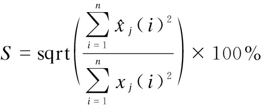
(12)
where ![]() represents the i-th sampling point of the j-th IMF of the extended signal, and xj(i) represents the i-th sampling point of the j-th IMF of the original signal. The closer to 100% the ρ is, the better the control effect of the end effect.
represents the i-th sampling point of the j-th IMF of the extended signal, and xj(i) represents the i-th sampling point of the j-th IMF of the original signal. The closer to 100% the ρ is, the better the control effect of the end effect.
② IMF orthogonality is defined as

(13)
The O value is used to measure the orthogonality level of each IMF. The smaller the O value, the better the orthogonality of IMF. In general, the O value does not exceed 0.06, which means that the end effect suppression of this method is effective[13].
The waveform shown in Fig.11 includes the original signal, mirror extension signal, RBF extension signal, and signal after the extension of the proposed method. The first 50 sampling points of the waveform shown in Fig.11 are part of the original signal. Among them, the mirror extension uses the method in Ref.[19], in which the extreme point closest to the end point is used as the mirror point to fold the signal to obtain the extended signal. The RBF extension uses the method in Ref.[19], and its parameters are set as: The quantity of input neurons is 150; the quantity of output neurons is 50; the target mean square error is 0.001; and the expansion speed is 3.22. It can be seen intuitively from Fig.11 that the mirror extension is directly folded at the mirror point, causing the signal at the near end to be consistent while the signal be at the far end does not match the original signal. The RBF extension can make the extension signal be as close to the original signal as possible. However, the discontinuous signal makes neural network training and prediction more difficult, and the extended waveform is not ideal. The method in this paper can effectively capture similar waveforms and adaptively extend them to the endpoints, which are more consistent with the original signals.
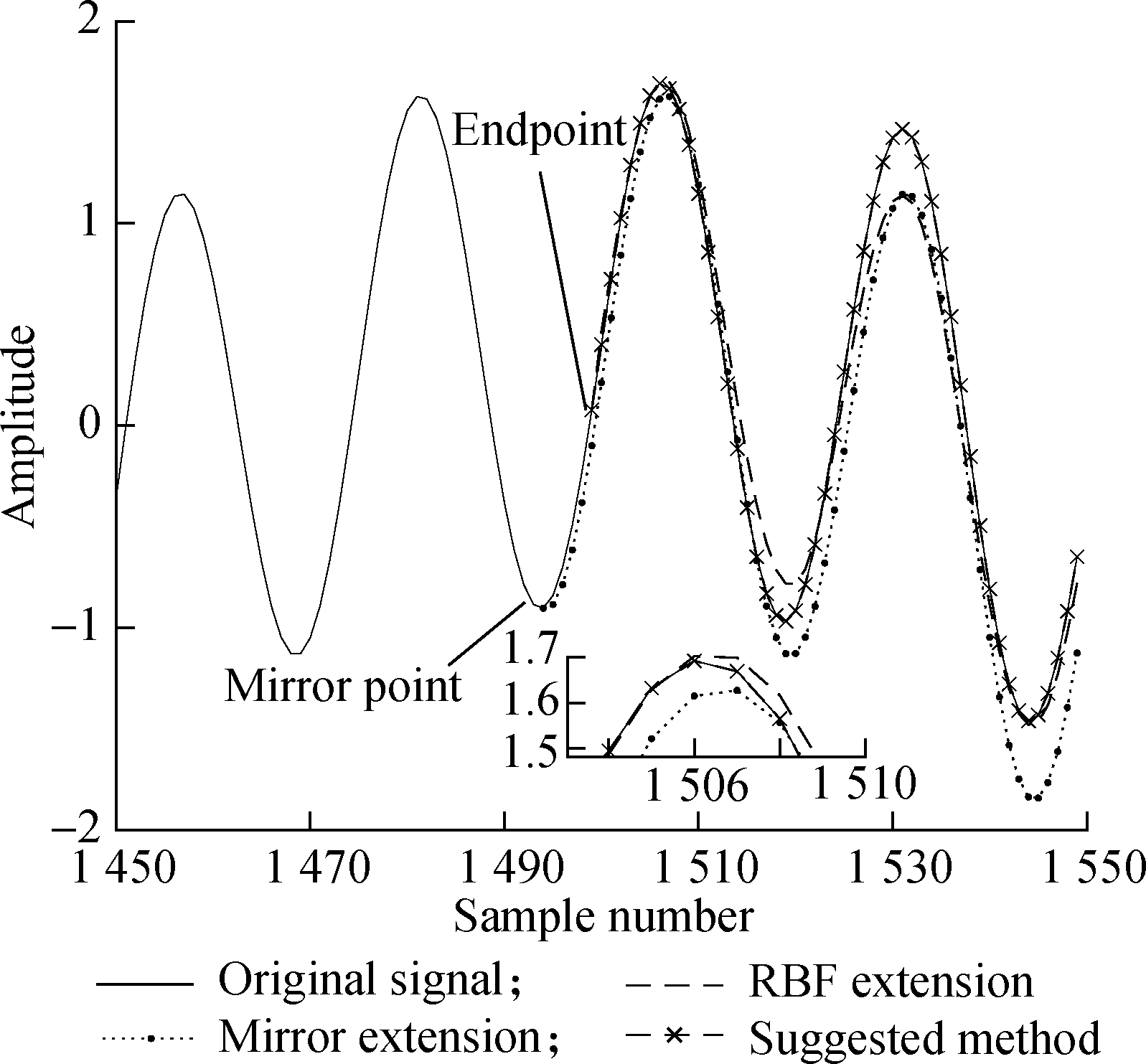
Fig.11 Results after the extension of various methods
The evaluation index values of various methods are shown in Tab.2. It can be seen intuitively that the unextended signal has a redundant IMF component, and its decomposition deviation gradually increases. The better the orthogonality level of the mirror extended signal, the more the third IMF begins to show a larger deviation. The neural network can better constrain the end effect after a short training, and the slight deviation is due to insufficient training time and training accuracy. Adjusting the training samples and training for a longer time can achieve higher accuracy. The proposed method has ideal indices because it directly predicts extended waveform according to the similar original signal to achieve a better control of the end effect, and it is effective and accurate.
Tab.2 Comparative analysis of evaluation indicators
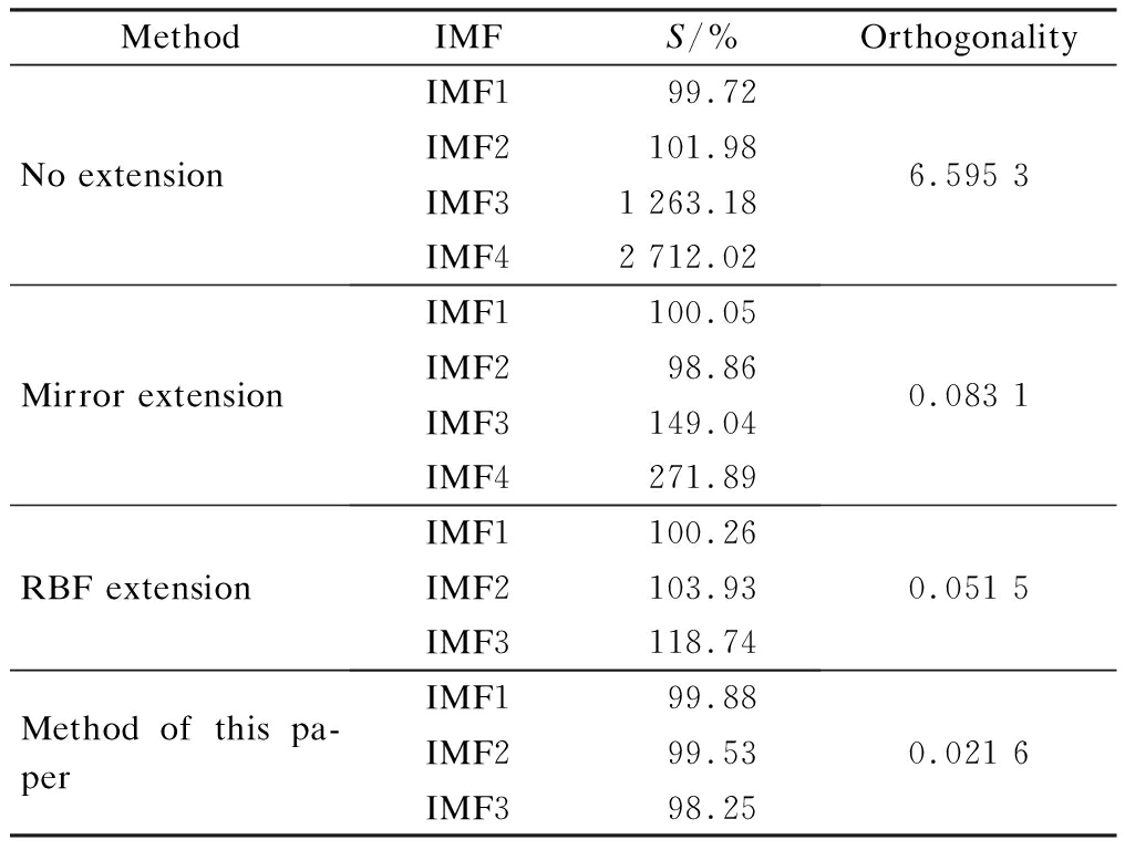
MethodIMFS/%OrthogonalityNo extensionIMF199.72IMF2101.98IMF31 263.18IMF42 712.026.595 3Mirror extensionIMF1100.05IMF298.86IMF3149.04IMF4271.890.083 1RBF extensionIMF1100.26IMF2103.93IMF3118.740.051 5Method of this pa-perIMF199.88IMF299.53IMF398.250.021 6
4 Test Signal Analysis
In order to further verify the practicability and effectiveness of the method,this paper uses the experimental device shown in Fig.12 to measure the faulty bearing signal. The bearing damage is processed on the outer ring, inner ring and rotor by EDM, and this paper randomly selects a section of the inner ring fault signal for analysis. The bearing model and experimental parameters are shown in Tab.3. The experimental signal is shown in Fig.13.
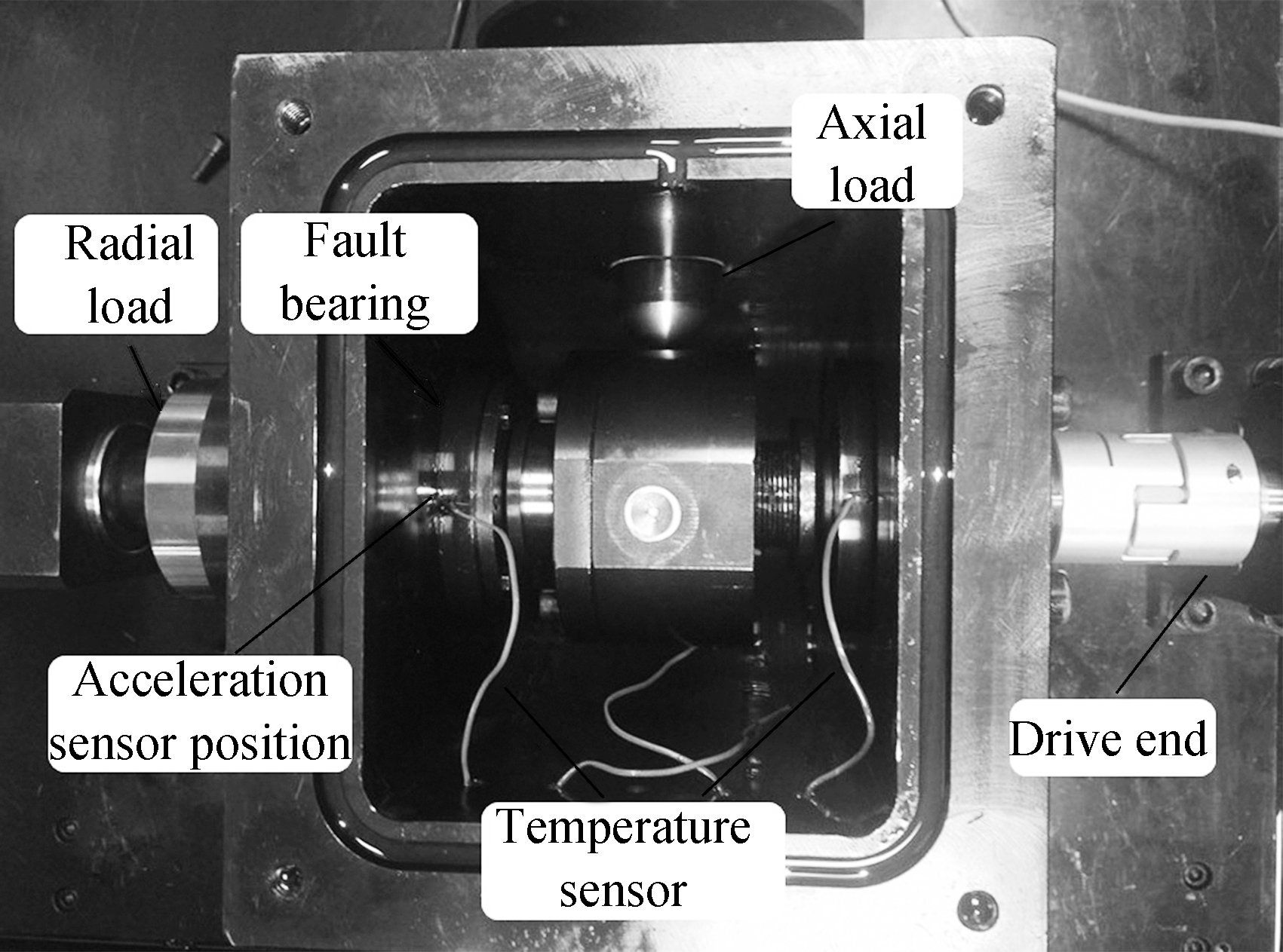
Fig.12 Experimental device
Tab.3 Bearing test parameters

Bearing typeSampling frequency/kHzRotating speed/(r·min-1)Damage size/mm6205244 0000.696

Fig.13 Experimental signal
The results of the direct EMD and the EMD extension by the above three methods are shown in Fig.14 to Fig.17, respectively. This paper only shows the first five modal components. Fig.14 shows that the signal via direct EMD has a serious end effect from IMF1 to IMF5. The target mean square error of the RBF extension is set to be 0.01 and other parameters are the same as in the previous section. It can be seen that the extension methods can better suppress the end effect, but IMF5 after mirror extension will perhaps diverge at the end of the signal.
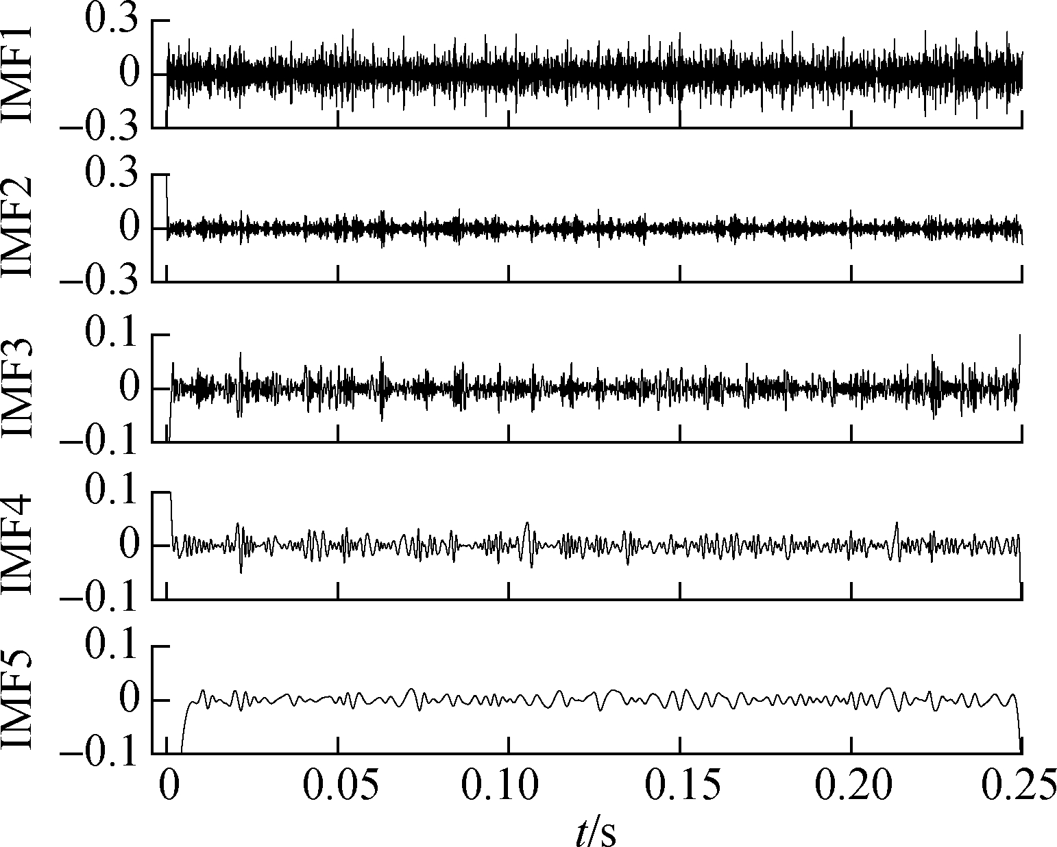
Fig.14 EMD results of unextended original signal
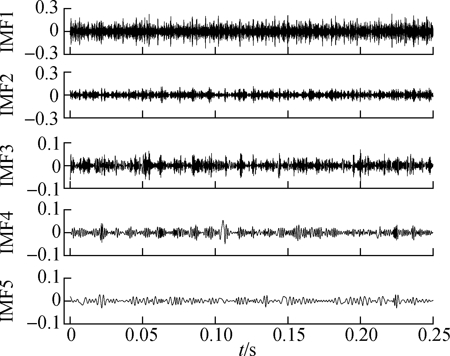
Fig.15 EMD results after mirror extension

Fig.16 EMD results after RBF extension
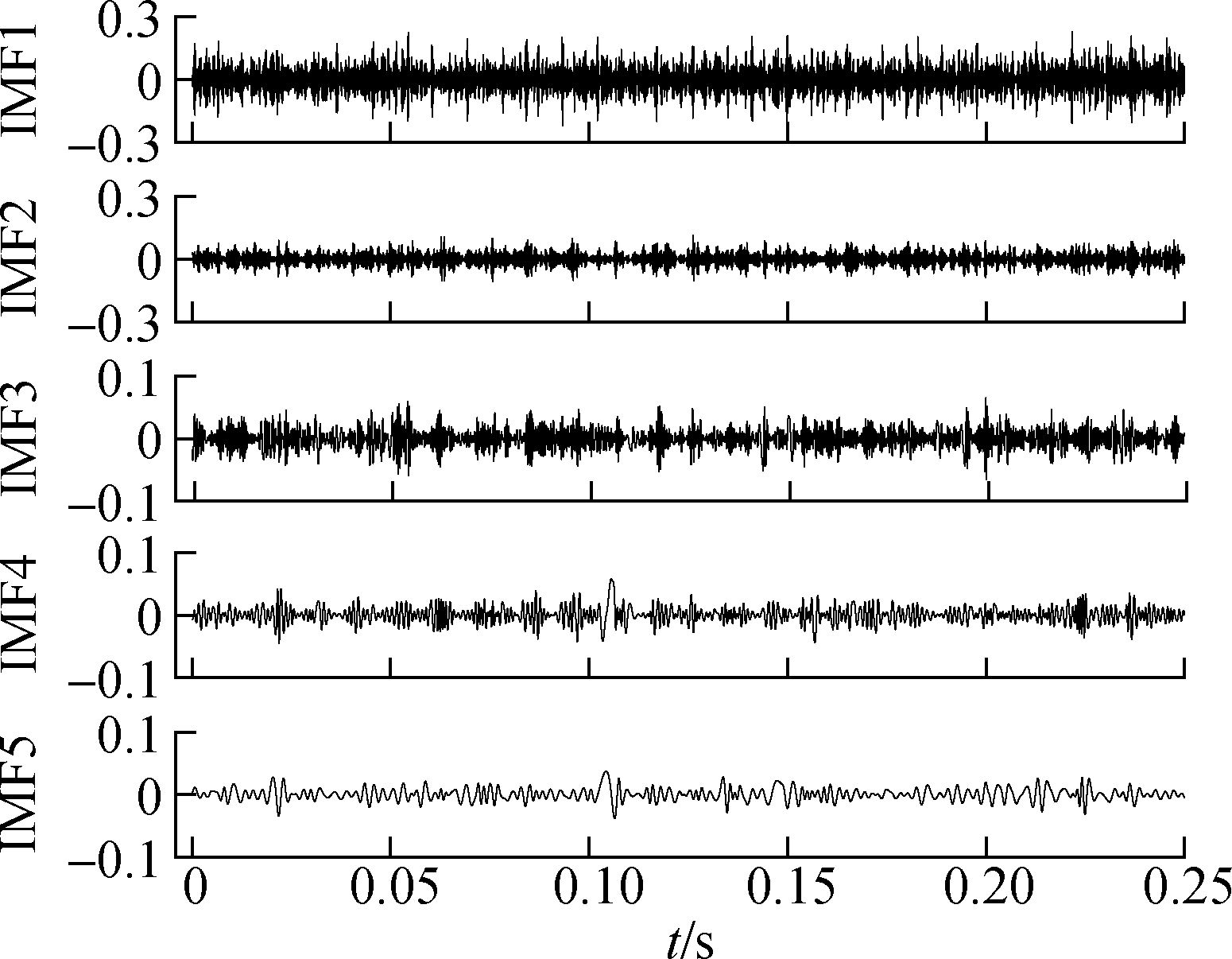
Fig.17 EMD results after the proposed extension
Two indices are also used to verify the effectiveness of the proposed method, and the comparative analysis results are listed in Tab.4. It can be seen that the EMD results similarity after mirror extension has a large deviation, the EMD results similarity after RBF extension is not stable enough, and the EMD results similarity after the proposed method has more consistent similarity with the original signal and a lower orthogonality index. Research results show that the proposed method is suitable for deterministic, stationary random and non-stationary random signals, and it has a good extension effect and is adaptive, so the proposed method can also provide some help for follow-up research.
Tab.4 Comparative analysis of evaluation indicator
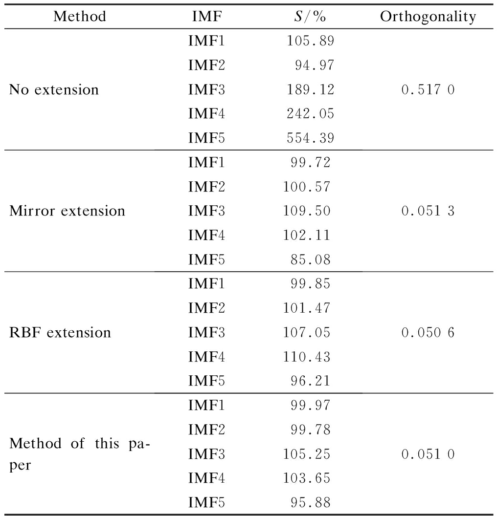
MethodIMFS/%OrthogonalityNo extensionIMF1105.89IMF294.97IMF3189.12IMF4242.05IMF5554.390.517 0Mirror extensionIMF199.72IMF2100.57IMF3109.50IMF4102.11IMF585.080.051 3RBF extensionIMF199.85IMF2101.47IMF3107.05IMF4110.43IMF596.210.050 6Method of this pa-perIMF199.97IMF299.78IMF3105.25IMF4103.65IMF595.880.051 0
5 Conclusions
1) The EMD end effect is analyzed based on the characteristics and shortcomings of the existing waveform matching and extension methods. An improved EMD end effect suppression method based on the sequential similarity and adaptive filter is proposed.
2) According to the simulation analysis and experimental data analysis, two evaluation indices show that the proposed method has some good effect on suppressing the EMD end effect which has a strong adaptability, accuracy and computational efficiency.
3) As the method needs to be given initial parameters in the adaptive prediction, its versatility is limited to a certain extent, and it needs further improvement for complete irregular signals in the future.
[1] Huang N E, Shen Z, Long S R, et al. The empirical mode decomposition and the Hilbert spectrum for nonlinear and non-stationary time series analysis[J]. Proceedings of the Royal Society of London Series A: Mathematical, Physical and Engineering Sciences, 1998, 454(1971): 903-995. DOI:10.1098/rspa.1998.0193.
[2] Huang N E, Shen Z, Long S R. A new view of nonlinear water waves: The Hilbert spectrum[J]. Annual Review of Fluid Mechanics, 1999, 31(1): 417-457. DOI:10.1146/annurev.fluid.31.1.417.
[3] Bi F R, Ma T, Wang X. Development of a novel knock characteristic detection method for gasoline engines based on wavelet-denoising and EMD decomposition[J].Mechanical Systems and Signal Processing, 2019, 117: 517-536. DOI:10.1016/j.ymssp.2018.08.008.
[4] Nie Z H, Shen F, Xu D J, et al. An EMD-SVR model for short-term prediction of ship motion using mirror symmetry and SVR algorithms to eliminate EMD boundary effect[J]. Ocean Engineering, 2020, 217: 107927. DOI:10.1016/j.oceaneng.2020.107927.
[5] Zhang X J, Huo Y, Wan D S. Improved EMD based on piecewise cubic hermite interpolation and mirror extension[J]. Chinese Journal of Electronics, 2020, 29(5): 899-905. DOI:10.1049/cje.2020.08.005.
[6] Yang J P, Li P Z, Yang Y F, et al. An improved EMD method for modal identification and a combined static-dynamic method for damage detection[J]. Journal of Sound and Vibration, 2018, 420: 242-260. DOI:10.1016/j.jsv.2018.01.036.
[7] Wang J, Liu W Y, Zhang S. An approach to eliminating end effects of EMD through mirror extension coupled with support vector machine method[J]. Personal and Ubiquitous Computing, 2019, 23(3/4): 443-452. DOI:10.1007/s00779-018-01198-6.
[8] Hao R J, Li F. A new method to suppress the EMD endpoint effect[J]. Journal of Vibration, Measurement and Diagnosis, 2018, 38(2): 341-345. DOI:10.16450/j.cnki.issn.1004-6801.2018.02.019. (in Chinese)
[9] Shao C X, Wang J, Fan J F, et al. A self adaptive method dealing with the end issue of EMD[J]. Acta Electtonica Sinica, 2007, 35(10): 1944-1948. (in Chinese)
[10] Su D L, Zheng H P. A boundary extension method for empirical mode decomposition end effect[J]. Journal of Aeronautics, 2016, 37(3): 960-969. (in Chinese)
[11] Xu Z F, Liu K. Method of empirical mode decomposition end effect based on analysis of extreme value symbol sequence[J]. Journal of Vibration, Measurement & Diagnosis, 2015, 35(2): 309-315. (in Chinese)
[12] Rong Q B. Research on EMD method for improving end effect and suppressing modal mixing [D]. Tianjin: Tianjin University, 2017. (in Chinese)
[13] Wald A. Sequential analysis[M]. New York: Wiley, 1947.
[14] Chen H X, Shang Y F, Sun K. Multiple fault condition recognition of gearbox with sequential hypothesis test[J].Mechanical Systems and Signal Processing, 2013, 40(2): 469-482. DOI:10.1016/j.ymssp.2013.06.023.
[15] Qian G B, Dong F, Wang S Y. Robust constrained minimum mixture kernel risk-sensitive loss algorithm for adaptive filtering[J].Digital Signal Processing, 2020, 107: 102859. DOI:10.1016/j.dsp.2020.102859.
[16] Zhu L F, Song C T, Pan L Z, et al. Adaptive filtering under the maximum correntropy criterion with variable center[J].IEEE Access, 2019, 7: 105902-105908. DOI:10.1109/ACCESS.2019.2932201.
[17] Li Y, Fang Z B, Wei Y F. Suppressing end effect of EMD based on local polynomial regression[J]. Journal of University of Science and Technology of China, 2014, 44(9): 786-792. (in Chinese)
[18] Huang N E, Wu M L C, Long S R, et al. A confidence limit for the empirical mode decomposition and Hilbert spectral analysis[J].Proceedings of the Royal Society of London Series A: Mathematical, Physical and Engineering Sciences, 2003, 459(2037): 2317-2345. DOI:10.1098/rspa.2003.1123.
[19] Han J P, Qian J, Dong X J. A method using mirror extension and RBF neural network to deal with end effect in EMD[J]. Journal of Vibration, Measurement & Diagnosis, 2010, 30(4): 414-417. (in Chinese)