Workpiece surface defects can reduce the strength of materials, shorten the life of workpieces, and increase safety-related risks[1]. Small defects are a part of the defects on the workpiece surface. They have great reference significance because they can reflect potential risks, such as the early failure of the production line and workpiece defects. However, given their small quantity and inconspicuous visual features, the detection of small defects is one of the problems in the field of workpiece surface quality inspection on the production line[2].
In the field of workpiece surface-defect detection, the earliest method is manual inspection, which consumes a considerable amount of manpower, and the inspection results are easily affected by the inspector subjectively. Therefore, new methods are proposed based on machine learning and machine vision[3]. Such methods usually include three steps: image preprocessing, feature extraction, and classification. Support vector machines[4], extreme learning machines[5], and artificial neural networks[6] have been used in these methods to realize the detection of workpiece surface defects. However, such methods cannot handle complex background images and detect multiple defects on one image.
In recent years, the convolutional neural network (CNN)[7] has been developed rapidly; it can be used in the field of target detection and segmentation. Target detection networks are divided into two categories, namely, one-stage and two-stage methods. The one-stage method includes YOLO[8] and SSD[9], and the two-stage methods mainly include region-based CNN (RCNN)[10] series. Several scholars applied these target detection networks to the detection of workpiece surface defects. Li et al. [11] proposed an improved YOLO network that can be used to detect six types of steel-strip surface defects. Wei et al.[12] designed a multi-scale deep CNN to detect various types of surface defects on aluminum profiles. Li et al.[13] introduced a method for detecting container surface defects based on the SSD network. Xue et al.[14] proposed a complex background defect detection method based on Faster-RCNN. Du et al.[15] improved the network’s detection performance on casting surface defects by combining feature pyramid networks and Faster-RCNN. However, the performance of the target detection network for small targets still needs to be improved, and the research on the detection of small defects needs further development.
Based on the above research, we propose a method named CSYOLOv3. This method is used to detect small defects on a workpiece surface. The CutMix[16] method is used to expand the training samples dynamically. The YOLOv3[17] is used for defect detection and optimized to focus on small defects. Firstly, the theoretical basis of the CutMix and YOLOv3 methods is briefly introduced in this paper. Secondly, the specific implementation of CSYOLOv3, including the sample enhancement method and optimization on YOLOv3, are explained. Then, the experiments and comparison with other methods are conducted to verifie the network performance.
1 Theoretical Basis of the Proposed Method
1.1 CutMix method
The CutMix method is a regularization strategy for the CNN classification model, and it performs sample transformation by cutting and splicing two training images. As shown in Fig. 1, a local area of a training image is removed, and the removed area is filled with a patch from another image. The category label of the image is mixed based on the area ratio of the original and patch images.
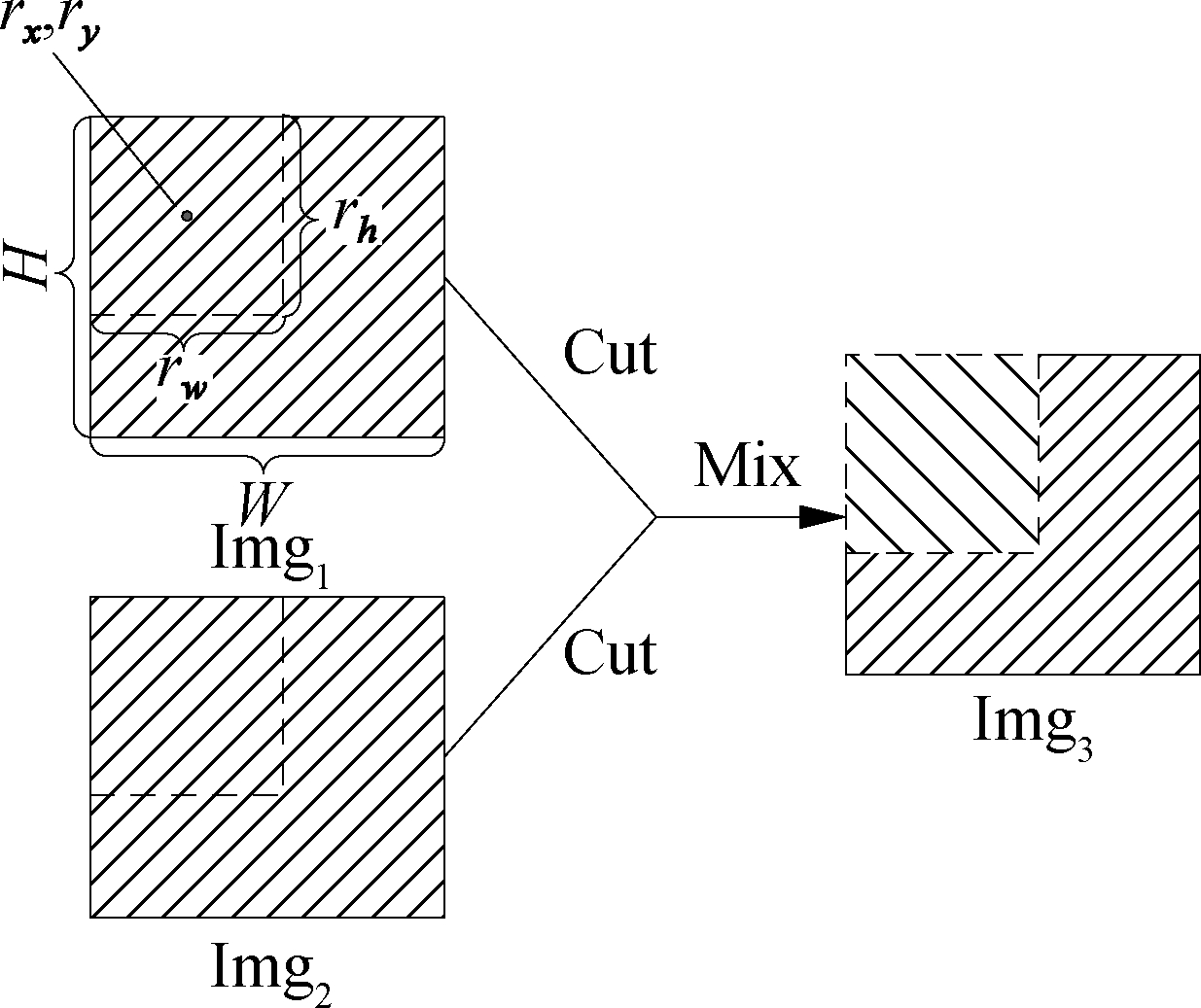
Fig.1 Schematic of CutMix method
1.2 YOLOv3 target detection network
YOLOv3 divides the image into s×s grids, and each grid is given k anchor boxes. YOLOv3 outputs a tensor of size s×s×[k×(5+v)], including the position (x,y), size (w,h), confidence C, and corresponding categories probability p(c). The labels of position and size are calculated as where (bx,by) are the real coordinates of the target boxes; (zx,zy) are the coordinates of the upper-left corner of the grids; and (bw,bh) and (aw,ah) denote the real sizes of the target and anchor boxes, respectively.
(1)
The true information of the prediction boxes can be obtained by performing the corresponding inverse transformation on the network output. The loss can be obtained by performing the corresponding error calculation between ![]() and (x,y,w,h).
and (x,y,w,h).
The DarkNet-53 classification network is used as the backbone network of YOLOv3 to extract image features, and YOLOv3 is used to perform multi-scale prediction on the extracted features. The prediction loss is divided into four parts, where the confidence error and category prediction error are defined by cross entropy, and the position and size errors are defined by the squared errors. The prediction loss can be calculated by the following:
![]()
![]()
(2)
where s is the quantity of grids in one direction; r is the number of anchor boxes on each grid; ![]() is the opposite; variables λnoobj and λcoord are constant weight coefficients.
is the opposite; variables λnoobj and λcoord are constant weight coefficients.
2 CSYOLOv3 Defect Detection Method
2.1 Dynamic method for training in sample expansion
One of the ways to improve the small-defect detection performance is by increasing the quantity and diversity of small defects in the training set. This paper designs a four-image stitching method based on the CutMix method and beta distribution. The method is used to enhance the training images and increase the small-defect training sample quantity. The beta distribution is used to adjust the balance between the original and enhanced samples because the excessive use of enhanced training samples will reduce the network’s generalization to the original samples, resulting in a decreased network performance.
Different from the CutMix, n2(n≥2) images are used to generate enhanced images in this paper to maximize the use of space on the image and avoid the considerable loss of defect features. In addition to the function of shrinking images, the method proposed in this paper can randomly transform defect locations and intercept part of the defects, which can improve the sensitivity of the network to the location and size of defects. This paper uses four images to generate enhanced samples. The use of additional images is unnecessary because as shown in Fig. 2, the four-image stitching-enhanced image after random flipping and
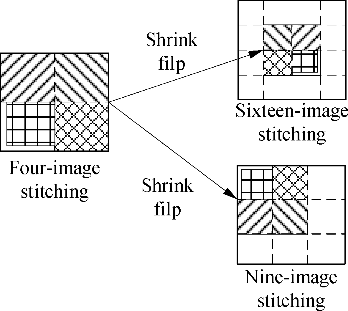
Fig.2 Operation diagram of random shrinking and flipping
shrinking operations can obtain the same characteristics originating from complex stitching. Thus, this paper uses the four-image stitching method combined with random flipping and shrinking instead of complicated image stitching.
As shown in Fig.2, four images are selected and zoomed out. The shrunk images are placed in the lower-right, lower-left, upper-right, and upper-left areas based on the center coordinate (sx,sy), which is randomly selected. After placement of the images, the empty area is filled with a gray value of 128. The shrinkage ratio is set to 0.5, that is, between 0.4 to 0.6, to ensure that the image will not be excessively shrunk. As shown in Fig. 3, to avoid the excessive cropping of images, the stitching center’s coordinates are selected using the following:
ε~Unif(0.4,0.6), sx=εW
λ~Unif(0.4,0.6), sy=λH
(3)
where ε and λ are the coefficients used to determine the splicing center; and W and H are the image width and height, respectively.
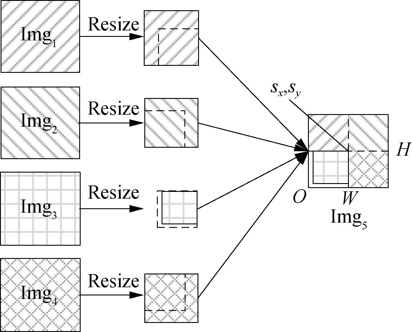
Fig.3 Schematic of the four-picture stitching method
After the sample is enhanced, the cutting and stitching of images will cause changes in the target boxes. Thus, the position and size of the target boxes are updated as new labels. Fig. 4 shows the update process of the training labels. The steps are as follows:
1) Four images are randomly selected from the training sample set, and the target box label is (xij,yij,wij,hij).
2) The image is shrunk by a certain ratio αk. The change in the target box is presented as
3) Based on the stitching center point (sx,sy), four images are placed on the generated image. The label change of the target box is as
4) Finally, whether the target box is truncated is assessed. If the target box is truncated, whether its short-side length is less than the threshold L is determined. If the short-side length is smaller than L, then the target box will be discarded; otherwise, the new position and size ![]() of the target box are generated.
of the target box are generated.
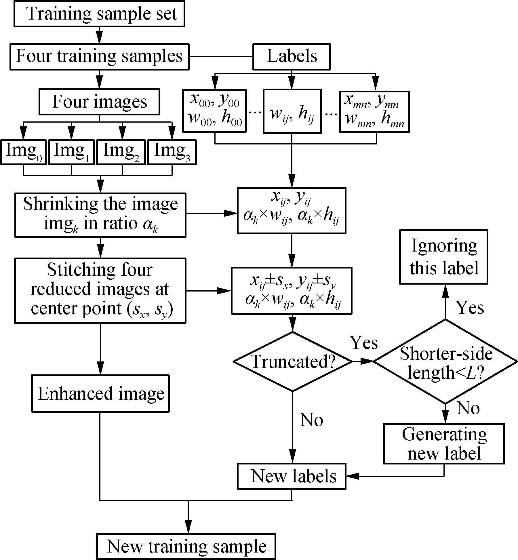
Fig.4 Flow chart of label update
As mentioned above, using enhanced training samples only is unreasonable. Therefore, the ratio between the expanded and original samples must be adjusted during training. The beta distribution is used for dynamic adjustment as
(4)
where m is the quantity of expanded samples that have been used in the current training; n is the quantity of original samples; η obeys the beta distribution. When ω=0, the original samples are used for training, and when ω=1, the expanded samples are generated and used for training.
2.2 Design of defect detection network
The deep DarkNet-53 network can extract rich semantic information. However, with the deepening of the network and shrinking of the feature map, the feature of small defects weakens gradually, which reduces the network performance in small-defect detection. The shallow and large feature maps contain a number of small-defect features. Thus, we split the large feature maps and send them to the detection branch for feature fusion. In this manner, the small-defect feature in the detection branch can be enriched, and the small-defect detection performance is improved.
As shown in Fig. 5, different from DarkNet-53, which uses a convolutional layer with a step size of 2 for feature map shrinking, maximum pooling is used to shrink the feature maps before feature fusion in the proposed method. The purpose is to retain the small-defect feature as much as possible. The network has three branches, and feature fusion processing is performed on each branch.
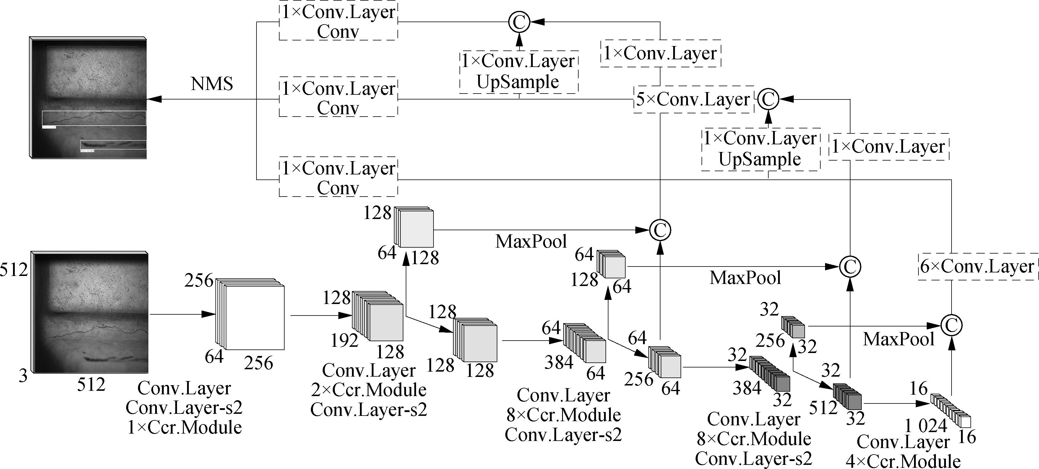
Fig.5 Structure of the improved YOLOv3
The overall network is based on the residual network[18]; the BN[19] layer is used to accelerate convergence and avoid overfitting. The linear activation function Leaky ReLu is used as the activation function. Fig. 6 shows the structure of Conv. Layer and Ccr. Module. The BN layer and activation function are placed behind the ordinary convolutional layer, whereas the Ccr.Module is composed of two convolutional layers, in which the 1×1 convolution kernel is used to fuse features from the channel direction, and the 3×3 convolution kernel is used to obtain large field features.

Fig.6 Structure of two main units in the improved YOLOv3
2.3 Loss function of the defect detection network
The position and size losses are separated in the loss function of YOLOv3, which easily causes two convergence processes to be asynchronous during training. Therefore, the GIoU[20] loss is used to combine the position and size losses. The calculation formula of GIoU value and the loss defined are listed as
lGIoU=1-VGIoU
(5)
where VIoU is the IoU value; VGIoU is the GIoU value; A and B are the areas of the target and prediction boxes, respectively; and E is the smallest closed area that can contain the prediction and target boxes.
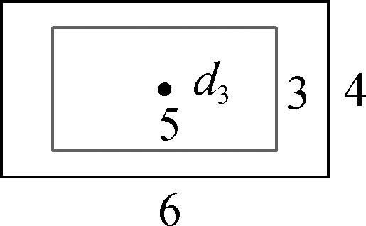
However, GIoU still presents several drawbacks. In specific cases, such as the target and prediction boxes, in a cross or containment relationship, GIoU cannot distinctly reflect the relative position of the two boxes. As shown in Fig. 7, the black box is the target box, and the gray box is the prediction box. From the comparison of the GIoU values of Figs. 7 (a) and (b) and those of Fig. 7 (c) and (d), the values of GIoU are equal, although the relative position of the two boxes is different. This drawback not only leads to the degradation of the network’s defect location performance but also reduces the network’s discrimination and classification performance due to the inaccurate selection of the defect area.
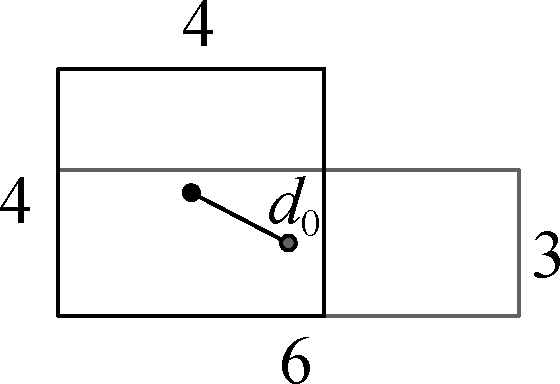
(a)
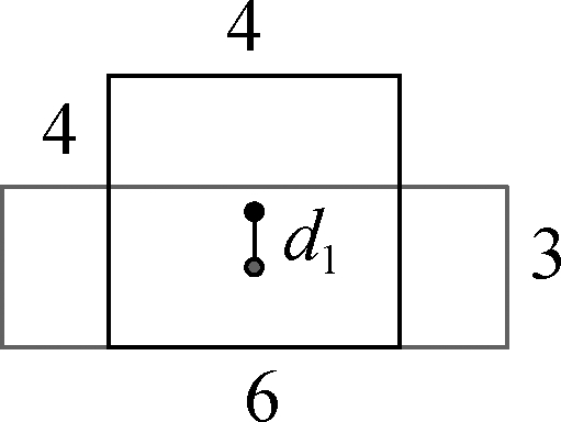
(b)
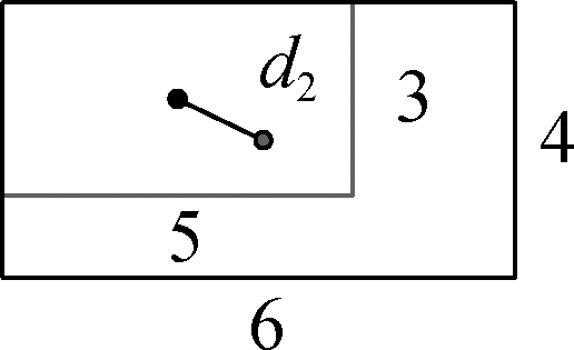
(c)
(d)
Fig.7 Comparison of GIoU values in different situations. (a) The first case of VGIoU=0.462; (b) The second case of VGIoU=0.462; (c) The first case of VGIoU=0.625;(d) The second case of VGIoU=0.625
This paper improves GIoU and calls it HIoU to solve the above problem. The area difference is used to enable HIoU to focus on the symmetry of the prediction box vertices, which is based on the center of the target box, thereby improving its positioning capability. The HIoU value VHIoU is calculated as
D=|Sru-Srd|+|Sru-Slu|
(6)
where Sruis the area of the box formed by the top-right vertices of the target and prediction boxes, namely, Srd and Slu, respectively, which are the areas formed by the bottom-right and top-left vertices.
The HIoU values of the four cases in Fig.7 are 0.462, 0.504, 0.583, and 0.625. HIoU exhibits an improved positioning performance. The loss function lHIoU is defined by VHIoU, and a cosine weight function related to the defect area is used to increase the network’s attention to small defects. The smaller the defect area, the larger the weight value. The lHIoUis calculated as
(7)
where u and v are the width and height of the target, respectively; and Sp is the image area.
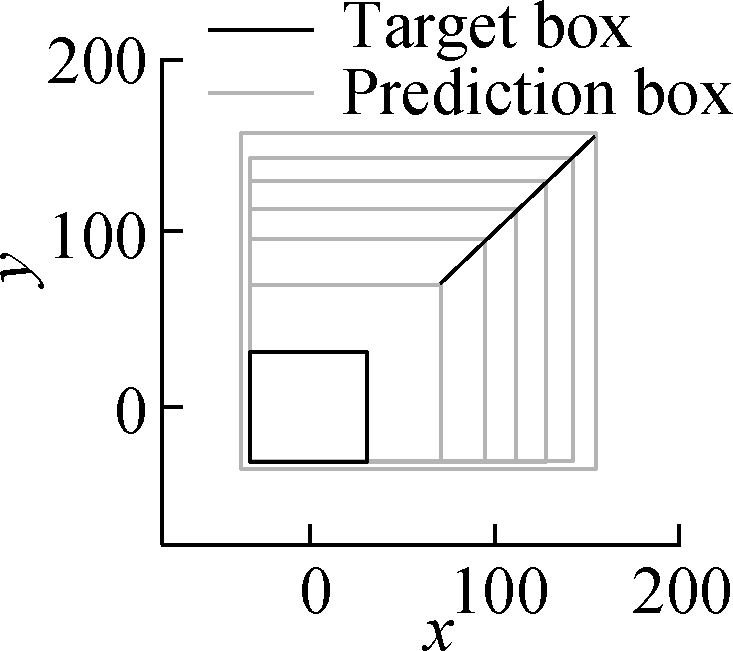
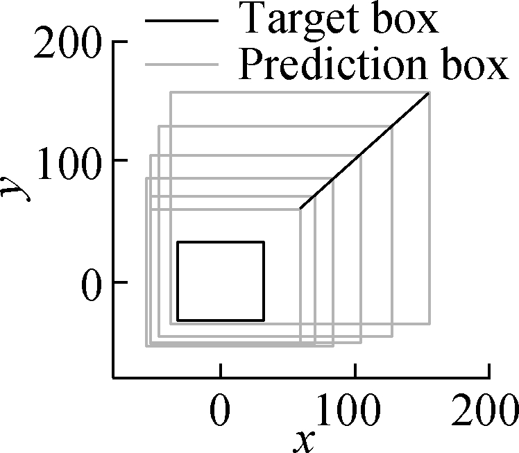
This paper simulates the reverse iterative process of the HIoU loss to verify its effectiveness. The losses of GIoU and YOLOv3 are used for comparison. A small 64×64 box is used as the target box, and a 192×192 box is used as the prediction box; the Adam iterator[21] is used for parameter optimization. The results are shown in Fig. 8, where the x-axis is the iteration times, and the y-axis denotes the IoU value after each iteration. The IoU value is between 0 and 1. The larger the IoU value, the more the prediction and target boxes overlap, implying an improved prediction accuracy. Our loss can reach a high IoU value in fewer iterations than the other two losses for a 64×64 small target box and a 192 × 192 prediction box. Thus, our loss substantially focuses on small targets, and the convergence process can be fast and accurate. Fig. 9 visualizes the change in the prediction box during the iteration process. Our loss function causes the complete overlap of the prediction and target boxes after 1 000 iterations, whereas the overlap areas of the other two losses are far smaller than ours.
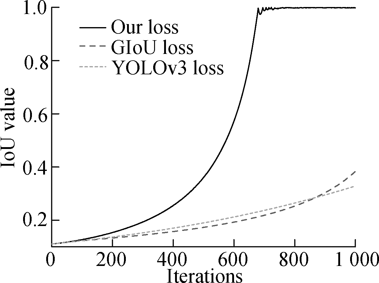
Fig.8 Iteration curve of the IoU value with different loss functions

(a)
(b)
(c)
Fig.9 Change in the prediction box during iteration. (a) Change with our loss; (b) Change with GIoU loss; (c) Change with YOLOv3 loss
3 Experiment
3.1 Dataset and experimental environment
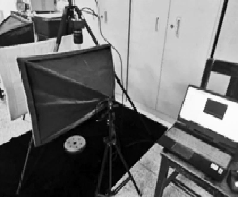
The experimental object is an aluminum workpiece casting, and an industrial charge-coupled device camera is used to collect surface-defect images. As shown in Fig. 10, the dark-field illumination is used as the illumination method, with the LED tube as the light source. The size of the collected image is 512 × 512 pixels, and 829 pictures are collected. The software LabelImg is used to mark the surface defects; and eight types of defects, including cracks, discoloration, insufficient pouring, fins, peeling, shrinkage holes, trachoma, and shrinkage porosity, are marked. The annotated images are divided into training, validation, and test sets at a ratio of 7∶1∶2.

(a)
(b)
Fig.10 Dark-field lighting and experimental site.(a) Schematic diagram of dark field illumination; (b) Picture of the experimental device
The computer used in the experiment is equipped with an Intel i7-8700 CPU and an RTX 2060Ti GPU. The software mainly includes python 3.7.2, DarkNet, Tensorflow 1.14, cuda10.2, and cuDNN7.6.
3.2 Parameter determination and network training
The K-means++ algorithm[22] is used to determine the quantity and size of the anchor boxes reasonably. The number of categories refers to the number of anchor boxes, and the center of each category after clustering is the size of the anchor box. The iteration termination condition of clustering is achieved when the results of two adjacent iterations are the same. The distance function is defined as follows:
D=1-VHIoU
(8)
As shown in Fig. 11, different numbers of anchor boxes are selected for the clustering experiments. As the quantity of anchor boxes increases, the average IoU increases rapidly in the early stage and then increases slowly after the number of boxes exceeds 9. Given that the increase in anchor box quantity will cause a substantial increase in the network parameters, 9 is selected as the number of anchor boxes to balance the amount of calculation and network performance. As shown in Fig. 12, the clustering results show that the sizes of the anchor boxes are (20×17), (74×18), (49×50), (213×28), (118×82), (235×47), (470×36), (465×61), and (270×167).
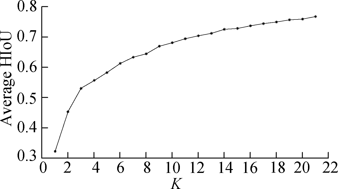
Fig.11 Clustering results under different numbers of anchor boxes
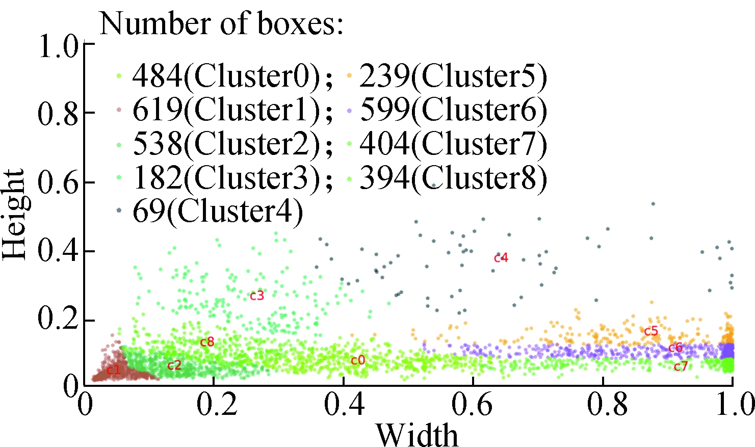
Fig.12 Clustering results with nine anchor boxes(Mean IoU is 0.664 2)
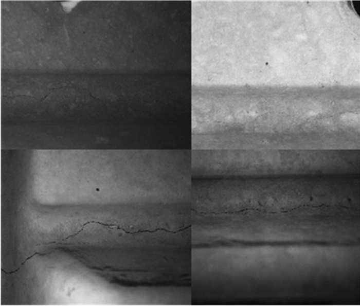
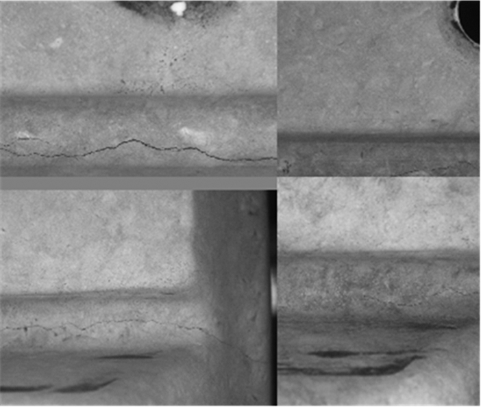
The network can be trained after the anchor boxes have been confirmed. The CutMix method with beta distribution is used to dynamically enhance the training samples in real time. Fig. 13 shows part of the enhanced training samples.
(a)
(b)
Fig.13 Two enhanced training images. (a) Enhanced training sample example 1; (b) Enhanced training sample example 2
The training batch size is 6. The cosine function is used as the learning rate, which decreases as the training frequency increases. The training termination condition is the completion of 2 000 epochs. The learning rate u is calculated as
(9)
where uinit is the initial learning rate; uend is the final learning rate; pglobal is the current iteration times; and ptotal is the total iteration times.
Fig. 14 shows the validation set loss curve in three cases, where the blue-green curve is the case observed without using the CutMix method, the magenta curve represents the case using the CutMix method without beta distribution, and the red curve denotes the case using the CutMix method with beta distribution. Compared with the other two curves, the red curve has a slower decline in the early stage, indicating that the CutMix method with beta distribution increases the diversity of the data set effectively. The red curve stabilizes at about 2.5, which is lower than those of the other two curves, indicating that the generalization capability of the network has been effectively improved. Fig. 15 shows each part of the validation set loss.
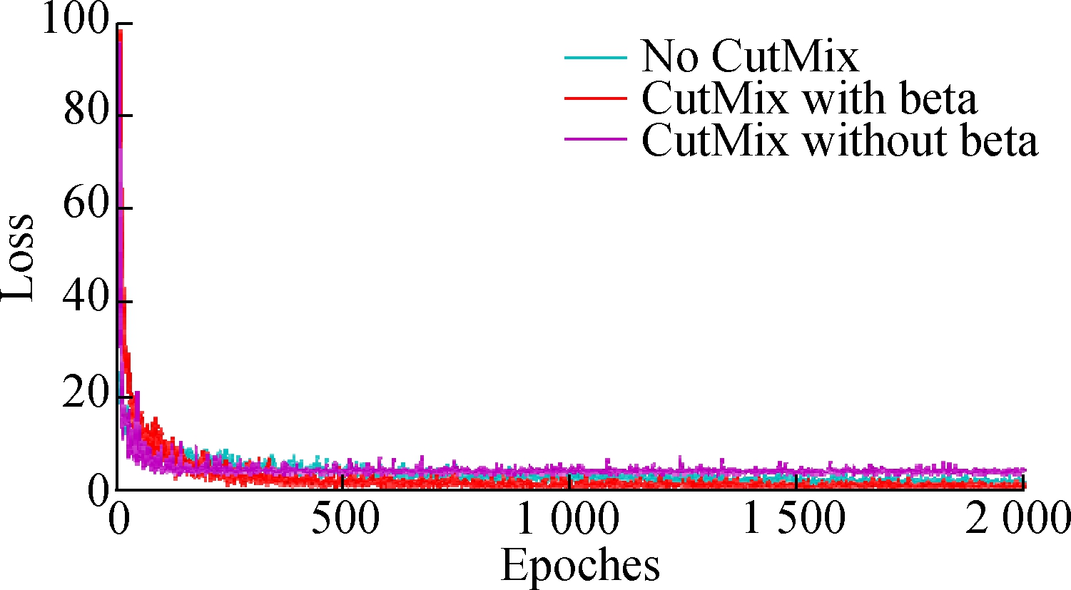
Fig.14 Validation set loss curve in three cases
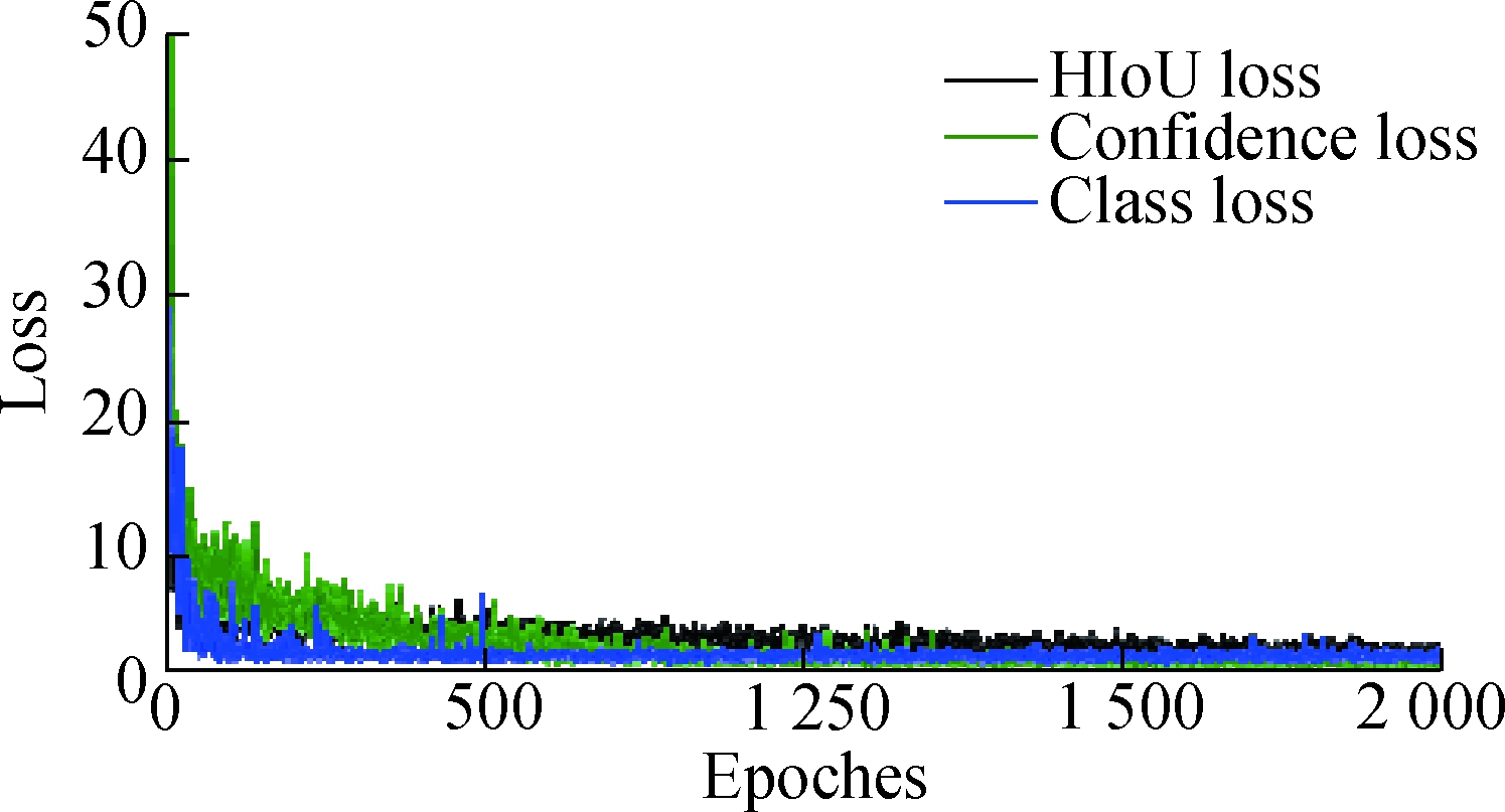
Fig.15 Change curve of different parts of validation set loss
3.3 Experimental results
After the network training is completed, the test set is used to test the network performance, and the performance is compared with those of YOLOv3, YOLOv3-GIoU, and Faster-RCNN[23]. The mAP[24-25] and speed are used as the performance indicators; mAP is the average of AP values of all categories, and speed is the number of images that the network can recognize per second. Tab.1 gives the comparison of the detection results of each method. The mAP value of our method is improved by 5%-10% compared with the other methods, and its speed can reach 14.09 frame/s with the RTX 2060Ti GPU. Thus, CSYOLOv3 can be used in dynamic detection during production when the time interval of workpiece production exceeds 70 ms.
Tab.1 Comparison of the detection results of each method

MethodmAP/%Speed/ frames-1 YOLOv361.7515.02YOLOv3-GIoU67.1915.02Faster-RCNN64.666.17CSYOLOv371.8014.09
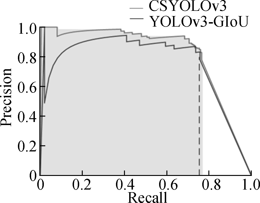
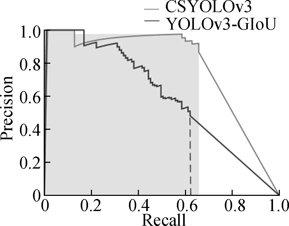
The largest defect size in the test set is 238 × 252. Thus, the defects are divided into three parts based on their area. These defects include small-scale defects with an area less than 64 × 64, medium-scale defects with an area between 64 × 64 and 128 × 128, and large-scale defects with an area between 128 × 128 and 256 × 256. The detection result of CSYOLOv3 is compared with that of YOLOv3-GIoU, which exhibits the best performance among the networks used for comparison. Tab. 2 shows the comparison of the AP value of CSYOLOv3 and YOLOv3-GIoU for different sizes of defects. CSYOLOv3 effectively improves the detection performance for different defect scales. The values in the table are the precision, recall, and AP values of two networks for different scales of defects. Compared with YOLOv3-GIoU, the AP value of CSYOLOv3 is increased by 13.93%, 7.37%, and 2.87% on the three defect scales.
Tab.2 Comparison of the AP value of CSYOLOv3 and YOLOv3-GIoU for different sizes of defects %

MethodSmall-scale defectsMedium-scale defectsLarge-scale defectsPRAPPRAPPRAPYOLOv3-GIoU48.2862.9750.2276.3877.1067.2388.6790.4687.98CSYOLOv386.7565.1564.1583.0277.3674.6090.3091.3290.85
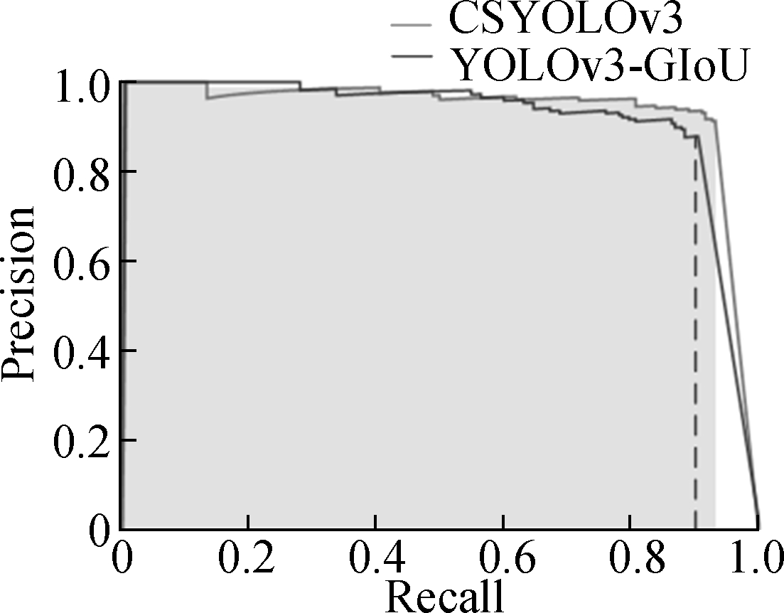
The AP curve of three scale defects is shown in Fig. 16, where the x-axis (recall) represents the percentage of defect quantity detected by the network to the actual defect quantity, and the y-axis (precision) represents the proportion of correct defect detection among the defects detected by the network. The AP value is the area of the shaded area in the figure. The gray curve is CSYOLOv3, and the black curve represents YOLOv3-GIoU.
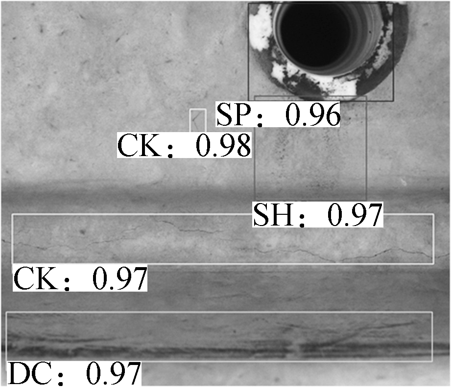
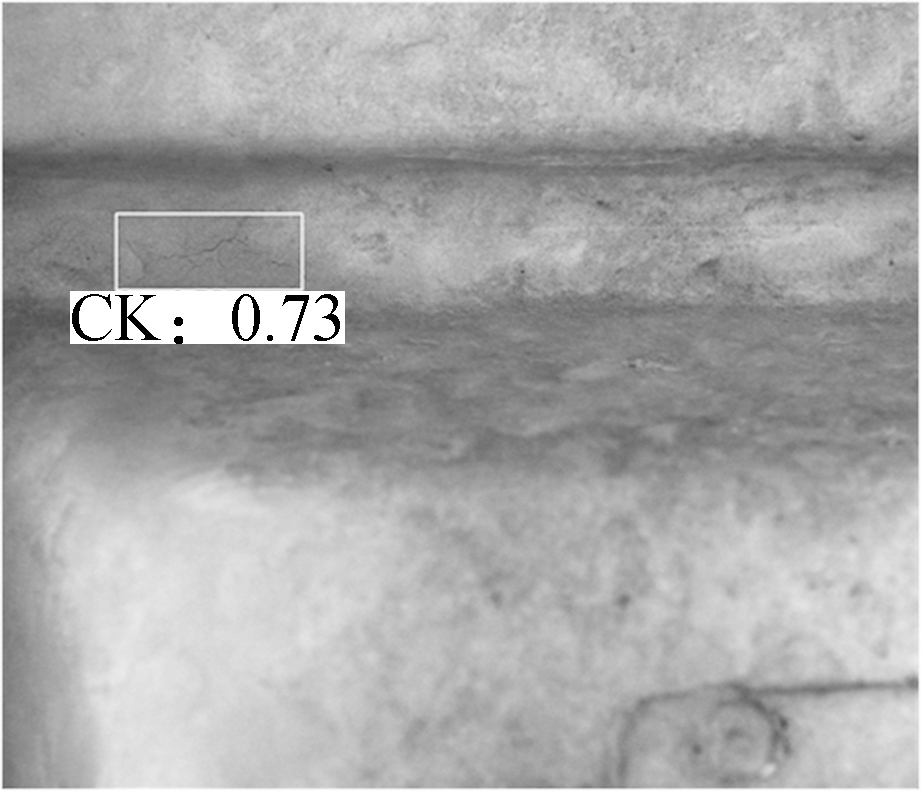
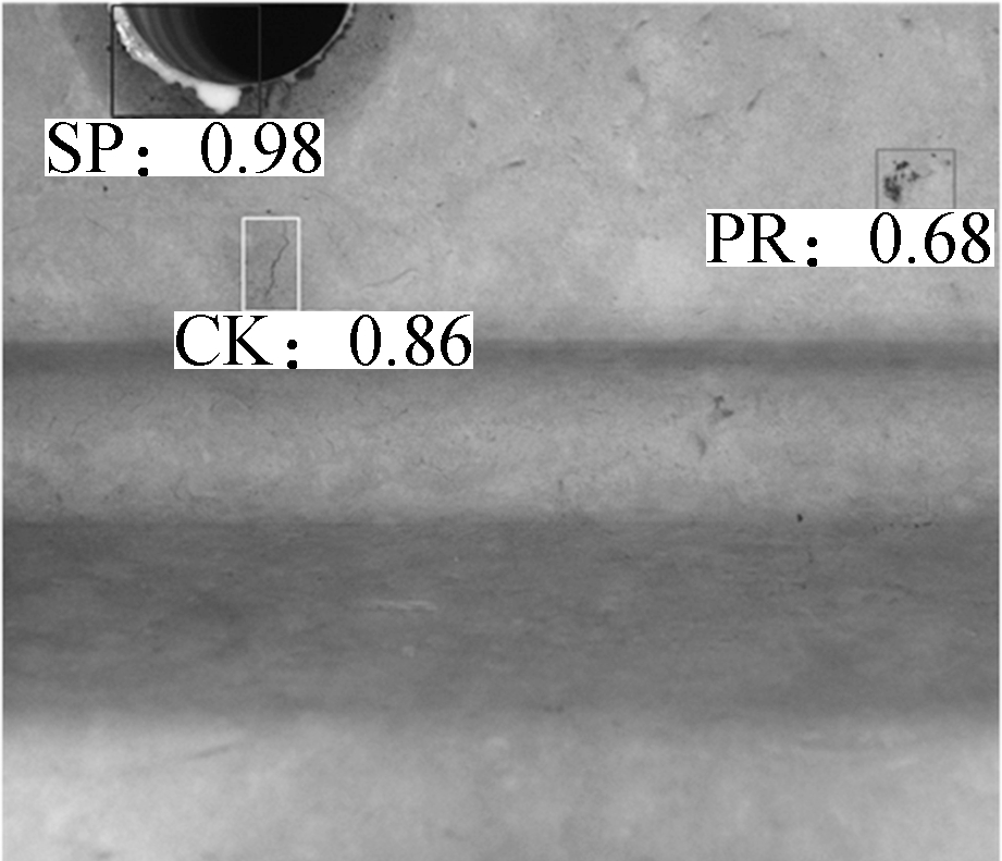
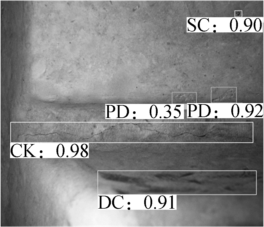
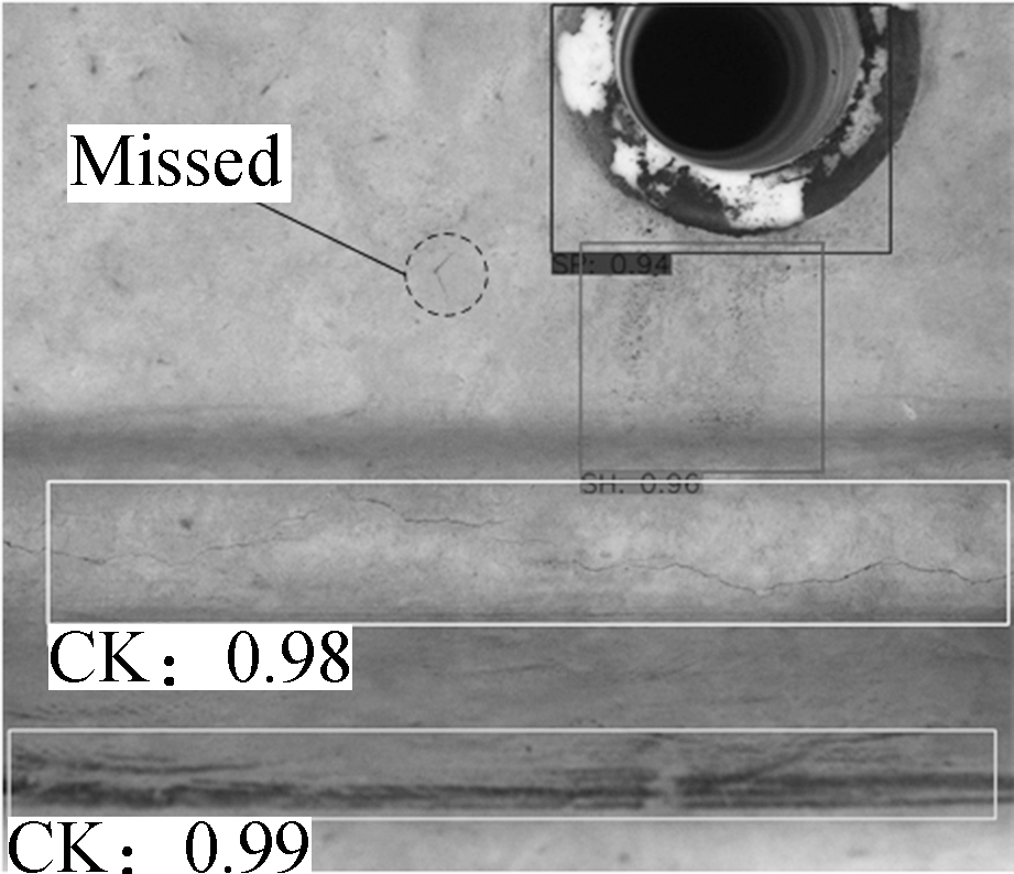
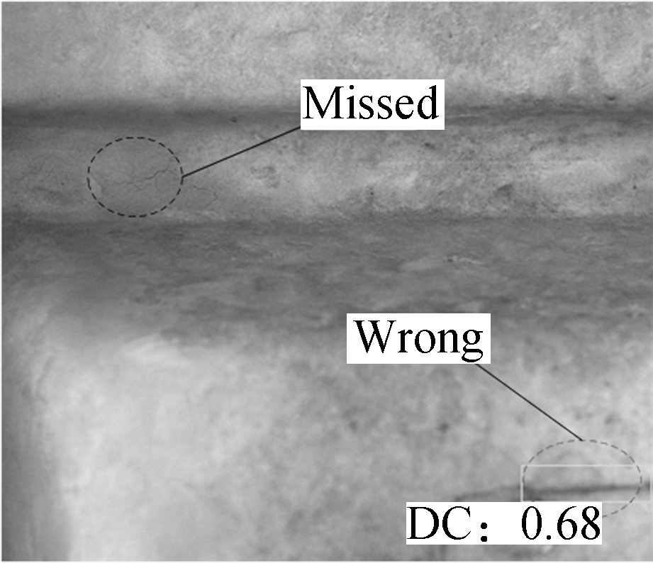
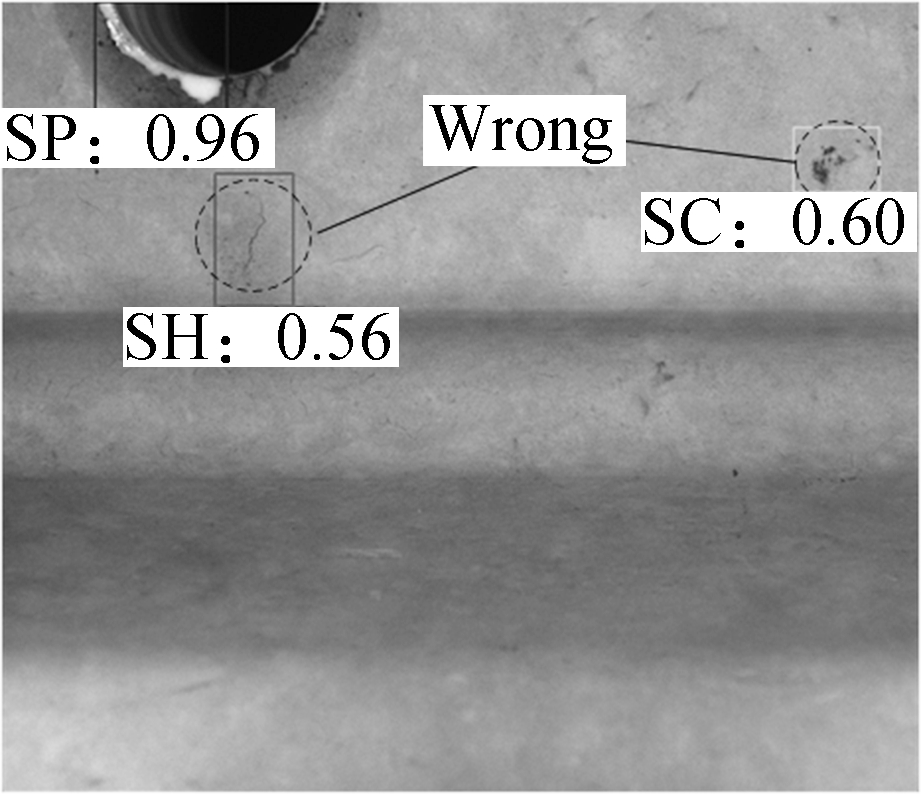
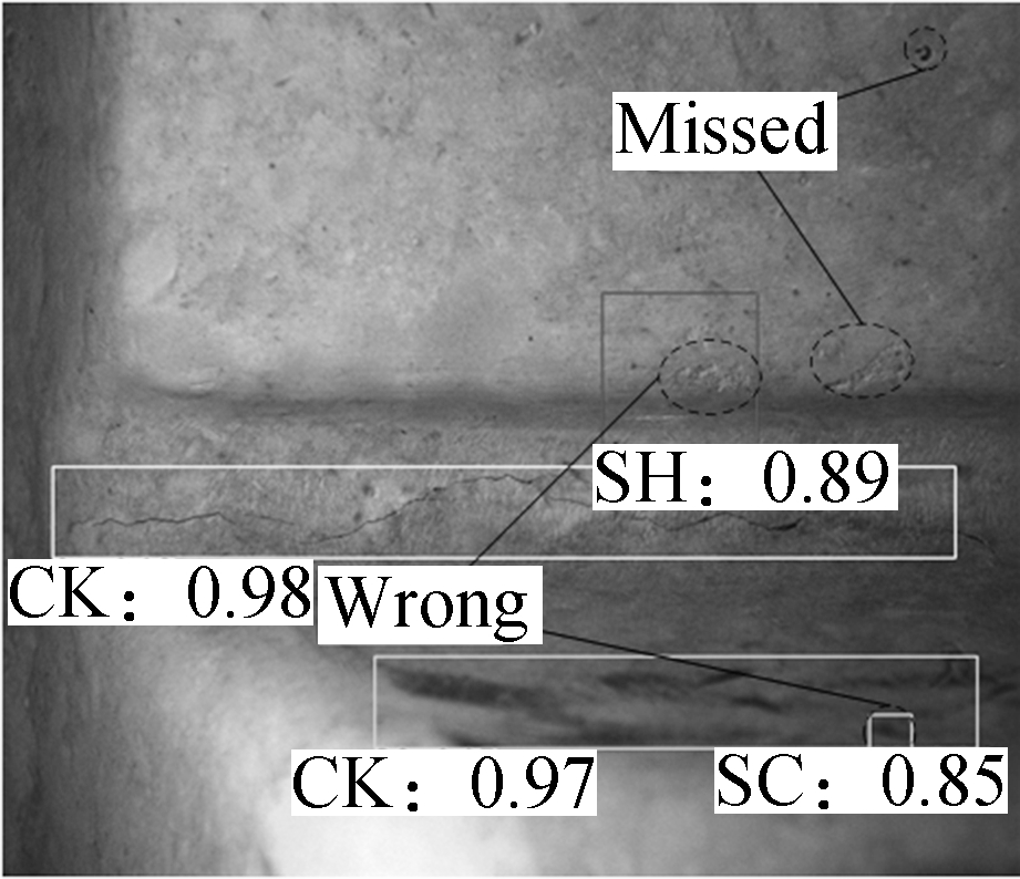
Fig. 17 shows part of the detection results of the two methods. The four images above are the results of CSYOLOv3, and the other four are those of YOLOv3-GIoU. CSYOLOv3 presents a better performance in the detection of small defects, which is manifested by a higher recognition rate and a lower error rate.
(a)
(b)
(c)
Fig.16 AP curve of different defect scales. (a) AP curve of large-scale defects; (b) AP curve of medium-scale defects; (c) AP curve of small-scale defects
(a)
(b)
(c)
(d)
(e)
(f)
(g)
(h)
Fig.17 Comparison of portions of the detection results. (a) Detection result of CSYOLOv3 on the first image; (b) Detection result of CSYOLOv3 on the second image; (c) Detection result of CSYOLOv3 on the third image; (d) Detection result of CSYOLOv3 on the fourth image; (e) Detection result of YOLOv3-GIoU on the first image; (b) Detection result of YOLOv3-GIoU on the second image; (c) Detection result of YOLOv3-GIoU on the third image; (d) Detection result of YOLOv3-GIoU on the fourth image
An additional experiment is conducted to test the relationship between the network performance and input image resolution. The test images are zoomed in before inputting to the network. Fig. 18 shows the network performance with different input resolutions. The abscissa is the resolution of the input image, and the ordinate is the AP value. The black curve represents the mAP value of all defects, and the grey curve shows the AP value of the small defects below 64 × 64 pixels on the original im-age. The performance of the network increases with the increase in image resolution. When the input image resolution is reduced to 224, and the small defects consequently shrunk below 28 × 28 pixels, the AP value of small defects is 32.46%, which can be regarded as an invalid detection. Therefore, the network is unsuitable for detecting small defects below 28 × 28 pixels.
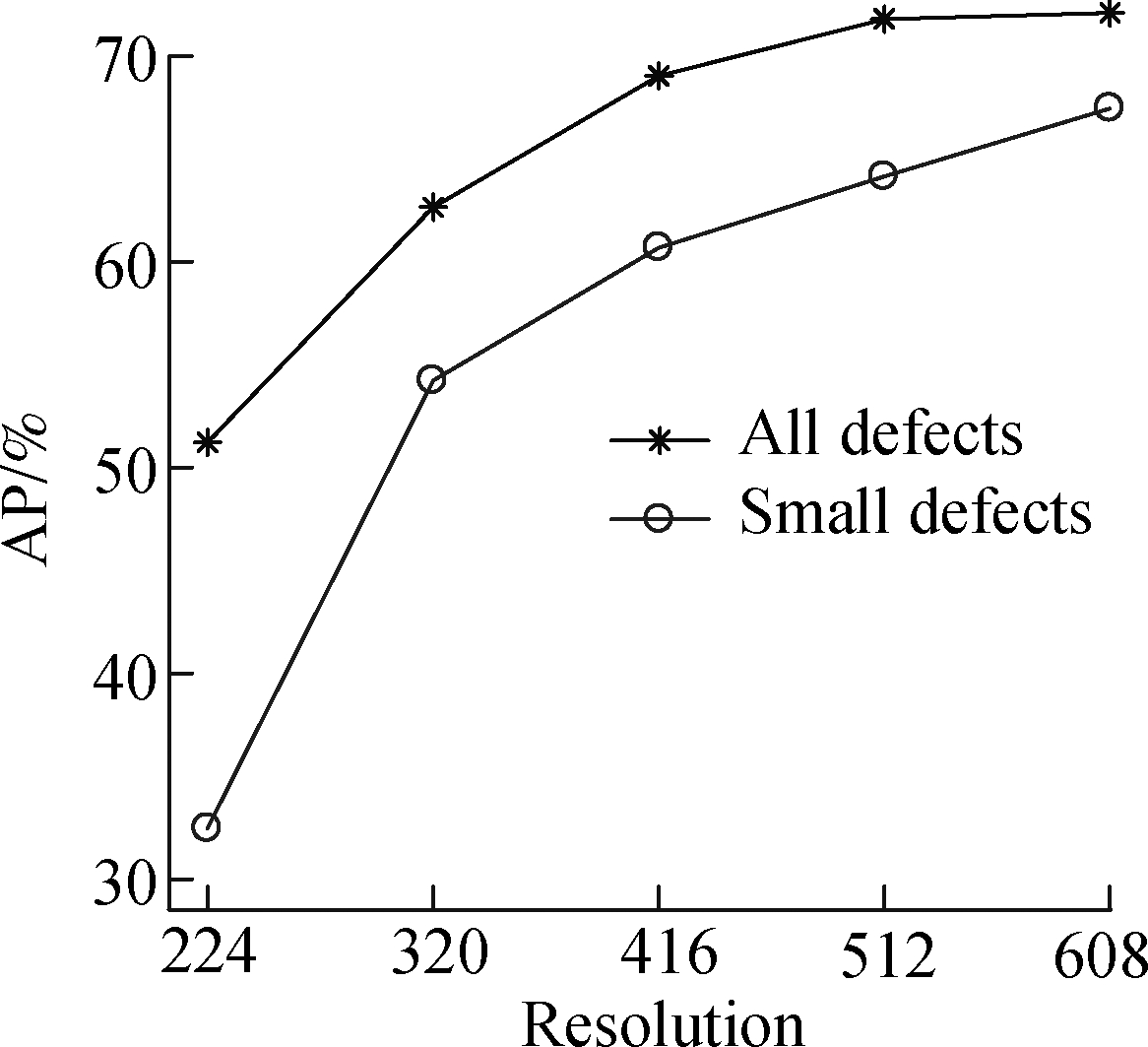
Fig.18 Network performance at different input resolutions
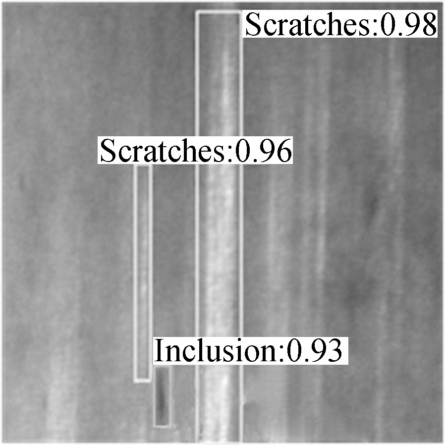
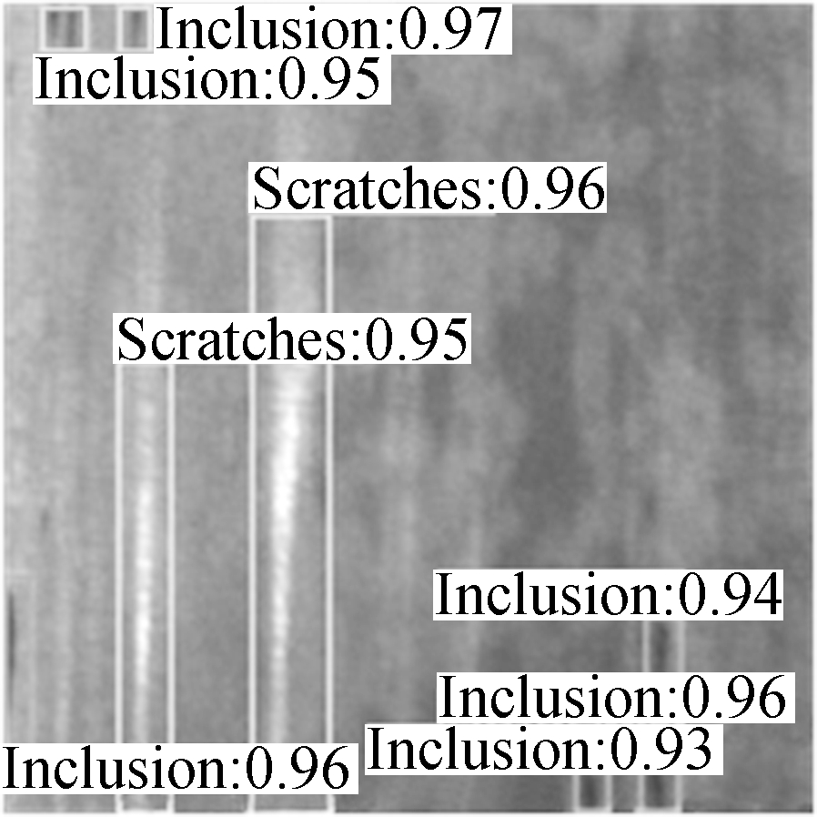
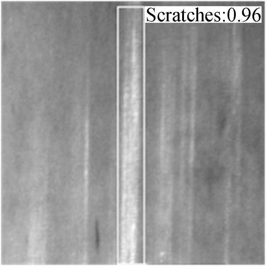
Experiments are conducted on the cold-rolled steel surface-defect data set NEU-DET to verify the universality of the method. Tab. 3 gives the detection performance of two networks. Our network works more effectively in detecting the surface defects of the cold-rolled steel. Fig. 19 shows part of the detection results, namely, those of CSYOLOv3 and YOLOv3-GIoU. CSYOLOv3 remains effective in detecting small surface defects on the cold-rolled steel.
Tab.3 Detection performance of two networks

MethodmAP/%Speed/ frames-1 YOLOv3-GIoU70.2528.12CSYOLOv375.5326.58
(a)
(b)
(c)

(d)
Fig.19 Comparison of the detection results on NEU-DT. (a) The first detection result of CSYOLOv3; (b) The second detection result of CSYOLOv3; (c) The first detection result of YOLOv3-GIoU; (d) The second detection result of YOLOv3-GIoU
4 Conclusions
1) The CutMix method with beta distribution effectively increases the quantity and diversity of small training defects, thus improving the small-defect detection performance.
2) The feature fusion of the improved YOLOv3 maintains the feature of small defects; the proposed HIoU is used to define the loss function, which improves the defect location capability. The loss is weighted, which enables the network to focus on small defects.
3) The proposed CSYOLOv3’s mAP reaches 71.80% at the speed of 14 frame/s, which is 5%-10% higher than that of other methods. For defects smaller than 64 × 64 pixels, the mAP increases by 14% compared with YOLOv3-GIoU. CSYOLOv3 has a better small-defect detection performance than the other methods.
4) This method is susceptible to environmental factors, such as oil covering the workpiece surface, insufficient or uneven light, and inaccurate lens focus, which affect the clarity of the captured image. This method has limitations in detecting defects with limited samples. Marking labels manifesting identification difficulty for each defect will be considered in future works.
[1]He Y, Song K C, Meng Q G, et al. An end-to-end steel surface defect detection approach via fusing multiple hierarchical features[J].IEEE Transactions on Instrumentation and Measurement, 2020, 69(4): 1493-1504. DOI:10.1109/TIM.2019.2915404.
[2]Sezgin M, Sankur B. Survey over image thresholding techniques and quantitative performance evaluation[J]. Journal of Electronic Imaging, 2004, 13(1): 146-165.
[3]Xu K, Xu Y, Zhou P, et al. Application of RNAMlet to surface defect identification of steels[J].Optics and Lasers in Engineering, 2018, 105: 110-117. DOI:10.1016/j.optlaseng.2018.01.010.
[4]You D Y, Gao X D, Katayama S. WPD-PCA-based laser welding process monitoring and defects diagnosis by using FNN and SVM[J].IEEE Transactions on Industrial Electronics, 2015, 62(1): 628-636. DOI:10.1109/TIE.2014.2319216.
[5]Liu Y, Xu K, Wang D D. Online surface defect identification of cold rolled strips based on local binary pattern and extreme learning machine[J].Metals, 2018, 8(3): 197. DOI:10.3390/met8030197.
[6]Vilar R, Zapata J, Ruiz R. An automatic system of classification of weld defects in radiographic images[J].NDT & E International, 2009, 42(5): 467-476. DOI:10.1016/j.ndteint.2009.02.004.
[7]Lecun Y, Bottou L. Gradient-based learning applied to document recognition[J]. Proceedings of the IEEE, 1998, 86(11):2278-2324.
[8]Redmon J, Divvala S, Girshick R, et al. You only look once: Unified, real-time object detection[C]//2016 IEEE Conference on Computer Vision and Pattern Recognition (CVPR). Las Vegas, NV, USA, 2016: 779-788. DOI:10.1109/CVPR.2016.91.
[9]Liu W, Anguelov D, Erhan D, et al. SSD:Single shot MultiBox detector[M]//Computer Vision—ECCV 2016. Cham: Springer International Publishing, 2016: 21-37. DOI:10.1007/978-3-319-46448-0_2.
[10]Girshick R, Donahue J, Darrell T, et al. Region-based convolutional networks for accurate object detection and segmentation[J].IEEE Transactions on Pattern Analysis and Machine Intelligence, 2016, 38(1): 142-158. DOI:10.1109/TPAMI.2015.2437384.
[11]Li J Y, Su Z F, Geng J H, et al. Real-time detection of steel strip surface defects based on improved YOLO detection network[J].IFAC-Papers OnLine, 2018, 51(21): 76-81. DOI:10.1016/j.ifacol.2018.09.412.
[12]Wei R F, Bi Y B. Research on recognition technology of aluminum profile surface defects based on deep learning[J]. Materials, 2019, 12(10): 1681.
[13]Li Y T, Huang H S, Xie Q S, et al. Research on a surface defect detection algorithm based on MobileNet-SSD[J].Applied Sciences, 2018, 8(9): 1678. DOI:10.3390/app8091678.
[14]Xue Y D, Li Y C. A fast detection method via region-based fully convolutional neural networks for shield tunnel lining defects[J].Computer-Aided Civil and Infrastructure Engineering, 2018, 33(8): 638-654. DOI:10.1111/mice.12367.
[15]Du W Z, Shen H Y, Fu J Z, et al. Approaches for improvement of the X-ray image defect detection of automobile casting aluminum parts based on deep learning[J].NDT & E International, 2019, 107: 102144. DOI:10.1016/j.ndteint.2019.102144.
[16]Yun S, Han D, Chun S, et al. CutMix: Regularization strategy to train strong classifiers with localizable features[C]//2019 IEEE/CVF International Conference on Computer Vision (ICCV). Seoul,South Korea, 2019: 6022-6031. DOI:10.1109/ICCV.2019.00612.
[17]Redmon J, Farhadi A. YOLOv3:An incremental improvement[EB/OL]. (2018)[2020-10-20]. https: //arxiv.org/abs/1804.02767
[18]He K M, Zhang X Y, Ren S Q, et al. Deep residual learning for image recognition[C]//2016 IEEE Conference on Computer Vision and Pattern Recognition (CVPR). Las Vegas, NV, USA, 2016: 770-778. DOI:10.1109/CVPR.2016.90.
[19]Ioffe S, Szegedy C. Batch normalization: Accelerating deep network training by reducing internal covariate shift[C]//International Conference on Machine Learning. Lille, France, 2015: 448-456.
[20]Rezatofighi H, Tsoi N, Gwak J, et al. Generalized intersection over union: A metric and a loss for bounding box regression[C]//2019 IEEE/CVF Conference on Computer Vision and Pattern Recognition (CVPR). Long Beach, CA, USA, 2019: 658-666. DOI:10.1109/CVPR.2019.00075.
[21]Han Z D. Dyna: A method of momentum for stochastic optimization[EB/OL]. (2018) [2020-10-20]. https: //arxiv.org/abs/1805.04933.
[22]Arthur D, Vassilvitskii S. K-means++: The advantages of careful seeding[C]//Proceedings of the Eighteenth Annual ACM-SIAM Symposium on Discrete Algorithms. Philadelphia, USA, 2007: 1027-1035.
[23]Ren S Q, He K M, Girshick R, et al. Faster R-CNN: Towards real-time object detection with region proposal networks[J].IEEE Transactions on Pattern Analysis and Machine Intelligence, 2017, 39(6): 1137-1149. DOI:10.1109/TPAMI.2016.2577031.
[24]Everingham M, van Gool L, Williams C K I, et al. The pascal visual object classes (voc) challenge[J]. International Journal of Computer Vision, 2010, 88(2): 303-338.
[25]Everingham M, Eslami S M A,van Gool L, et al. The pascal visual object classes challenge: A retrospective[J]. International Journal of Computer Vision, 2015, 111(1): 98-136. DOI:10.1007/s11263-014-0733-5.