The attitude and heading reference system (AHRS) plays an important role in carriers, such as vehicles, ships, and unmanned aerial vehicles[1-3]. The AHRS obtains the Euler angle of a carrier on the basis of the comparison of the rotation vectors of the carrier and the Earth for the measurement of the heading angle. One of the applications of the AHRS is the combination of inertial measurement units (IMUs) and magnetometers.
The approaches to calibrating magnetometers are very mature, and they are able to meet basic accuracy requirements[4-5]. The magnetic heading information of a three-axis magnetometer relative to the direction of the magnetic north is one of the most important parameters in navigation [6-8]. However, accurate heading estimation is not easy to conduct as it is often affected by many factors, which can be divided into two categories, namely, system errors and external interferences[9-12]. System errors include manufacturing and installation errors, and they can be mitigated by proper field calibration. As for external interferences, the approach to address them remains an open issue. For example, magnetic interference sources, such as ferromagnetic materials, machinery, and high voltage lines, are difficult to model in many unknown environments[13-16].Therefore, specific approaches need to be developed to reduce or eliminate magnetic field interference.
A number of approaches have been presented to mitigate the effects of external magnetic field disturbances on magnetic heading[17-18]; they can be divided into two broad categories, namely, data fusion of multiple sensor signals and compensation approaches using only magnetometer signals. The Kalman filter and its improved algorithm are the most commonly used algorithms to improve the accuracy of heading estimation by combining signals from multiple sensors, such as gyroscopes, accelerometers, and magnetometers. When magnetic disturbances occur, minimal weight is assigned to magnetometers, and the heading estimation depends heavily on gyroscopes and accelerometers[19-21].
In this study, we focus on the calculation of the heading angle on the basis of IMUs and magnetometers under magnetic interference. The novelties of this work are as follows. A calculation formula, including one for the heading angle, is established. The magnetometer and IMU are combined according to weight to calculate the heading angle on the basis of an error model. A random forest (RF) algorithm is used to determine the weight factor. The approach combines the advantages of two sensors and makes the final heading angle accurate and stable.
1 Methods
Firstly, a magnetic heading compensation approach is presented.Secondly, a fusion approach that combines the IMU and magnetometer to calculate the heading angle is proposed. Such a fusion approach is introduced in the following four sections.
1.1 Coordinate system conversion
Define two horizontal components of a geomagnetic field as Mx and My. Therefore, the magnetic heading can be calculated as If the magnetometer is horizontal,then we do not need to consider the vertical direction. Only the data of the X-axis and Y-axis can be used to calculate the heading an-gle. However, the magnetometer does not always maintain a horizontal direction during carrier movement. Thus, the magnetic field strength of the X-axis measured by the magnetometer is not a horizontal component.
(1)
The navigation coordinate system is a local cartesian coordinate system, and it rotates in the order of the ZXY axis. The attitude matrix is obtained as follows:

(2)
where ![]() is the attitude matrix of the carrier coordinate system relative to the navigation coordinate system; ψ is the yaw angle; θ is the pitch angle; γ is the roll angle.
is the attitude matrix of the carrier coordinate system relative to the navigation coordinate system; ψ is the yaw angle; θ is the pitch angle; γ is the roll angle.
1.2 Calculation of yaw angle
In this work, the dynamic direction angle approach based on a magnetometer is mainly divided into the following steps. Firstly, the error model of the magnetometer is established according to the error source of the magnetometer measurement. Secondly, a set of formulas containing the course angle information is obtained. Finally, the heading angle is obtained by solving the formula.
The sources of magnetometer errors include the magnetometer itself and external interferences. The errors caused by the magnetometer itself are unchanged with the external environment and can be mitigated by proper field calibration. The errors caused by external interferences are changeable with the external environment. Thus, the error model of the magnetometer can be expressed as follows:
(3)
where ![]() is the output vector of the magnetometer;
is the output vector of the magnetometer; ![]() is the matrix of the total error; Mb is the vector of the local magnetic field; mb is the error vector of zero offset; E is the error vector of the external environment; E0 is the error vector of measurement, which is generally considered to be white Gaussian noise and can thus be ignored.
is the matrix of the total error; Mb is the vector of the local magnetic field; mb is the error vector of zero offset; E is the error vector of the external environment; E0 is the error vector of measurement, which is generally considered to be white Gaussian noise and can thus be ignored.
Without the consideration of white Gaussian noise, the error model of the magnetometer can be simplified as
(4)
where ![]() is the output vector of the calibrated magnetometer.
is the output vector of the calibrated magnetometer.
If ![]() then Eq.(4) is expressed as
then Eq.(4) is expressed as
(5)
where N is the inverse matrix of the total error matrix, which remains unchanged with the external environment.
The matrix setting is introduced with consideration of the vertical direction. The correspondences of the magnetometer triaxial output at two adjacent time periods are expressed as
C1X1=C2X2
(6)
where C1 and C2 are the attitude matrices of two adjacent time periods; X1 and X2 are the triaxial output vectors of two adjacent time periods.
The aforementioned triaxial correspondence is expressed as
(7)
where ![]() is the calibrated output of the magnetometer.
is the calibrated output of the magnetometer.
If the carrier is in a horizontal position,then the force on the three axes is {0,0,-1}T. Combined with the output of the accelerometer,

(8)
where Ax, Ay, and Az are the outputs of the accelerometer.
From Eq.(8), the following can be obtained:

(9)
Then, θ and γ can be calculated as follows:
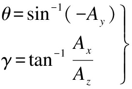
(10)
As each coordinate maintains a Cartesian coordinate system in the equivalent rotation of the b-to-n-system, ![]() It can be calculated according to Eq. (7) as
It can be calculated according to Eq. (7) as
(11)
It can also be calculated according to Eq. (5) as
NMh(k+1)-NE(k+1)
(12)
Therefore,
(13)
If ![]() and NE(k+1)={n1,n2,n3}T, then it can be calculated as follows:
and NE(k+1)={n1,n2,n3}T, then it can be calculated as follows:
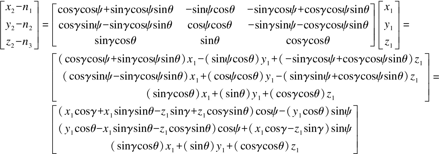
(14)
where {x1,y1,z1}T is the output of the magnetometer at the current time; {x2,y2,z2}T is the output of the magnetometer in the next time period; {n1,n1,n1}T is the interference on three axes.
Assuming a very small sampling time, the strengths of the magnetic fields at the adjacent time periods are nearly equal. That is, ‖Mk‖=‖Mk+1‖, and then ‖N(Mh-E)‖k=‖N(Mh-E)‖k+1. As the value at k is known, let ‖Mk‖=M0. Then,

(15)
(16)
According to Eqs. (14) and (16), and (sinψ)2+(cosψ)2=1, ψ can be calculated.
1.3 Weighted fusion approach based on IMU and magnetometer
The Kalman gain is affected by the process noise covariance (Q) and measured noise covariance (R). As the external magnetic field interference cannot be predicted, the values of Q and R are uncertain. Therefore, this study adopts the weighted fusion algorithm. The process of calculating the optimal value is presented in Fig. 1. The measured value of the magnetometer is adopted as the observed value AM(k), and the measured value of the IMU is adopted as the increment value U(k). The optimal value ![]() is calculated by Eq.(18). Then, AM(k) and
is calculated by Eq.(18). Then, AM(k) and ![]() are weighted to determine the optimal value A(k) at time k. At the next moment, the k time optimal value A(k) and U(k+1) are used to obtain the predicted value
are weighted to determine the optimal value A(k) at time k. At the next moment, the k time optimal value A(k) and U(k+1) are used to obtain the predicted value ![]() at k+1 time because the gyroscope is not as susceptible to the interference of the magnetic field in the environment as the magnetometer. Then, with AM(k+1), the k+1 time optimal value A(k+1) is obtained, and so on. In addition, the magnetometer provides the initial direction for the data conversion of the INS. When k=0, A(k)=AM(k) . When k≥1,
at k+1 time because the gyroscope is not as susceptible to the interference of the magnetic field in the environment as the magnetometer. Then, with AM(k+1), the k+1 time optimal value A(k+1) is obtained, and so on. In addition, the magnetometer provides the initial direction for the data conversion of the INS. When k=0, A(k)=AM(k) . When k≥1,
(17)
where AM(k) is the observation value of the magnetometer at time k; pk is the weight factor at time k.
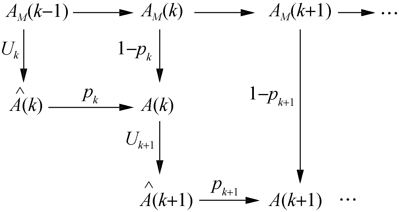
Fig.1 Process of calculating the optimal value
1.4 Weight optimization based on random forest algorithm
In this work, an RF algorithm is used to determine the weight factor pk. The RF algorithm is an integrated learning algorithm that is based on decision trees. It features a high prediction accuracy, good tolerance to outliers and noise, and resistance to overfitting. Given the interference information when the magnetometer and IMU collect data, the weighted fusion approach based on the RF algorithm can restore as much of the true angle as possible. In the calculation, ![]() and Ae(k) are selected as the characteristics of the RF decision tree. Large amounts of data are generated from random movements in buildings, and they are organized into datasets D={(x1,y1),(x2,y2),…,(xN,yN)}, where
and Ae(k) are selected as the characteristics of the RF decision tree. Large amounts of data are generated from random movements in buildings, and they are organized into datasets D={(x1,y1),(x2,y2),…,(xN,yN)}, where ![]() The calculation process of pk is shown in Fig.2.
The calculation process of pk is shown in Fig.2.
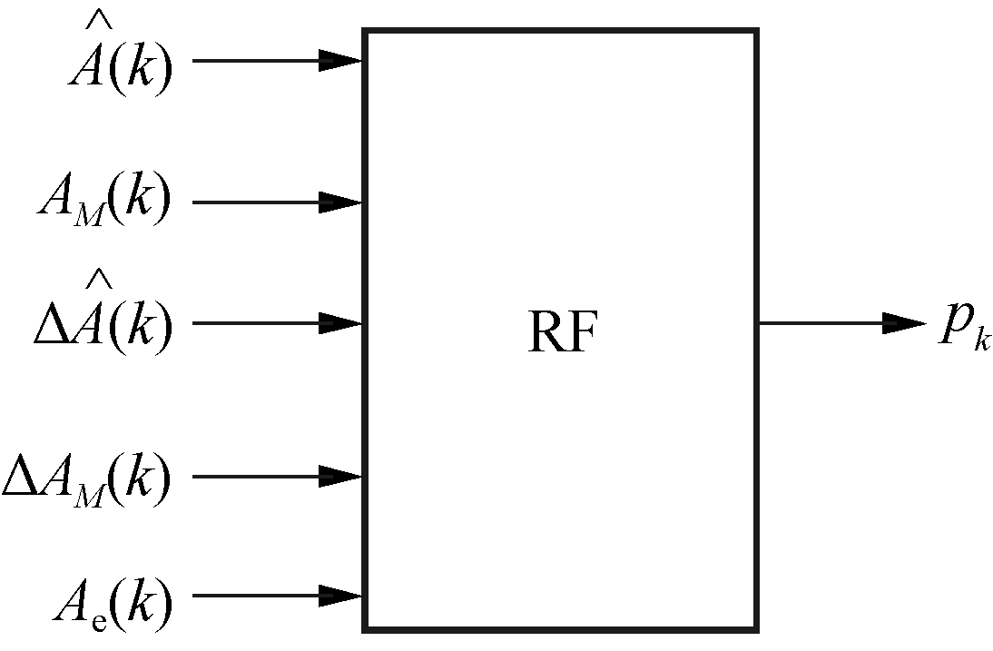
Fig.2 Prediction model of weight factor pk based on RF algorithm
The calculation method for the unknown component of x is as follows:

(18)
where ![]() and ΔAM(k) represent changes in the yaw angles per unit time; Ae(k) represents the deviation between the magnetometer measurements and the IMU calculations and reflects the disturbance of the magnetometer so as to reduce the weight of the output value of the magnetometer when the disturbance is too strong.
and ΔAM(k) represent changes in the yaw angles per unit time; Ae(k) represents the deviation between the magnetometer measurements and the IMU calculations and reflects the disturbance of the magnetometer so as to reduce the weight of the output value of the magnetometer when the disturbance is too strong.
The weight factor pk of each group of data can be calculated as follows:

(19)
The RF algorithm is divided into four steps. Firstly, samples are selected randomly. Secondly, characteristics are selected randomly. Thirdly, a decision tree (classification and regression tree) is constructed. Finally, RF voting (i.e., averaging the output of each decision tree) is performed. The core step of the RF algorithm is to build a decision tree. In this process, the cut points of each node and the final output values should be established.
The feature space division of each tree adopts a heuristic method. Each division examines all the values of all the features in the current set and selects the optimal one as the segmentation point according to the square error minimization criterion. The j-th feature variable x(j) and its value in the training are set as a cut variable and cut point respectively. Then, define two regions as R1(j,s)={x|x(j)≤s} and R2(j,s)={x|x(j)>s}. The best j and s are obtained by solving the following:
(20)
where c1 and c2 are the fixed output values in the two regions after division that minimize the square errors in each region. Obviously, these two optimal output values are the mean values of yi in their corresponding regions. After solving j and s, each region is recursively divided into two subregions, and j′ and s′ in each subregion are determined. The steps are repeated until the decision tree is constructed. The decision tree divides the input space into u regions R1,R2,…,Ru, and its output is as follows:
(21)
In the actual operation, the RF algorithm averages the results of each decision tree to obtain the current weight factor pk. Each phase of the calculation dynamically adjusts pk according to the situation of the previous phase. Hence, the divergence of heading angle errors caused by the long-term dependence on gyroscopes and accelerometers is avoided under interference.
2 Results
Magnetic field calibration is adopted to eliminate the zero errors of a magnetometer. The magnetometer measures the magnetic field strength of three axes. The direction of the magnetometer changes with carrier movement. The data measured by the sensor should have the same value in the positive and negative directions of the magnetic field; meanwhile, the symbols are opposite. In other words, the data should be a circle centered at the origin. This feature shows the zero drift of the data.
2.1 Results for heading angle calibration of magnetometer
The experiment for the heading calibration of the magnetometer is performed with a magnetic interference source nearby. A magnet is used as the interference source (red dot in Fig. 3). Path A is 0.1 m away from the interference source, and Path B is 0.6 m away from the interference source.
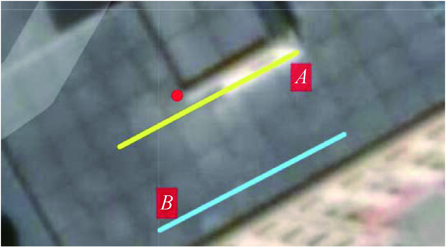
Fig.3 Testing of magnetometer calibration
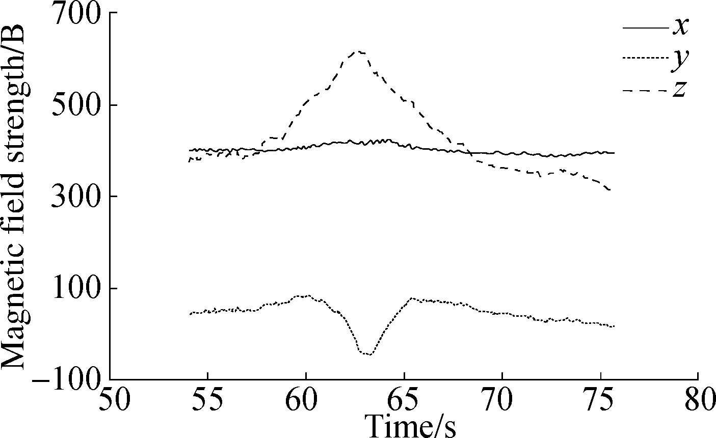
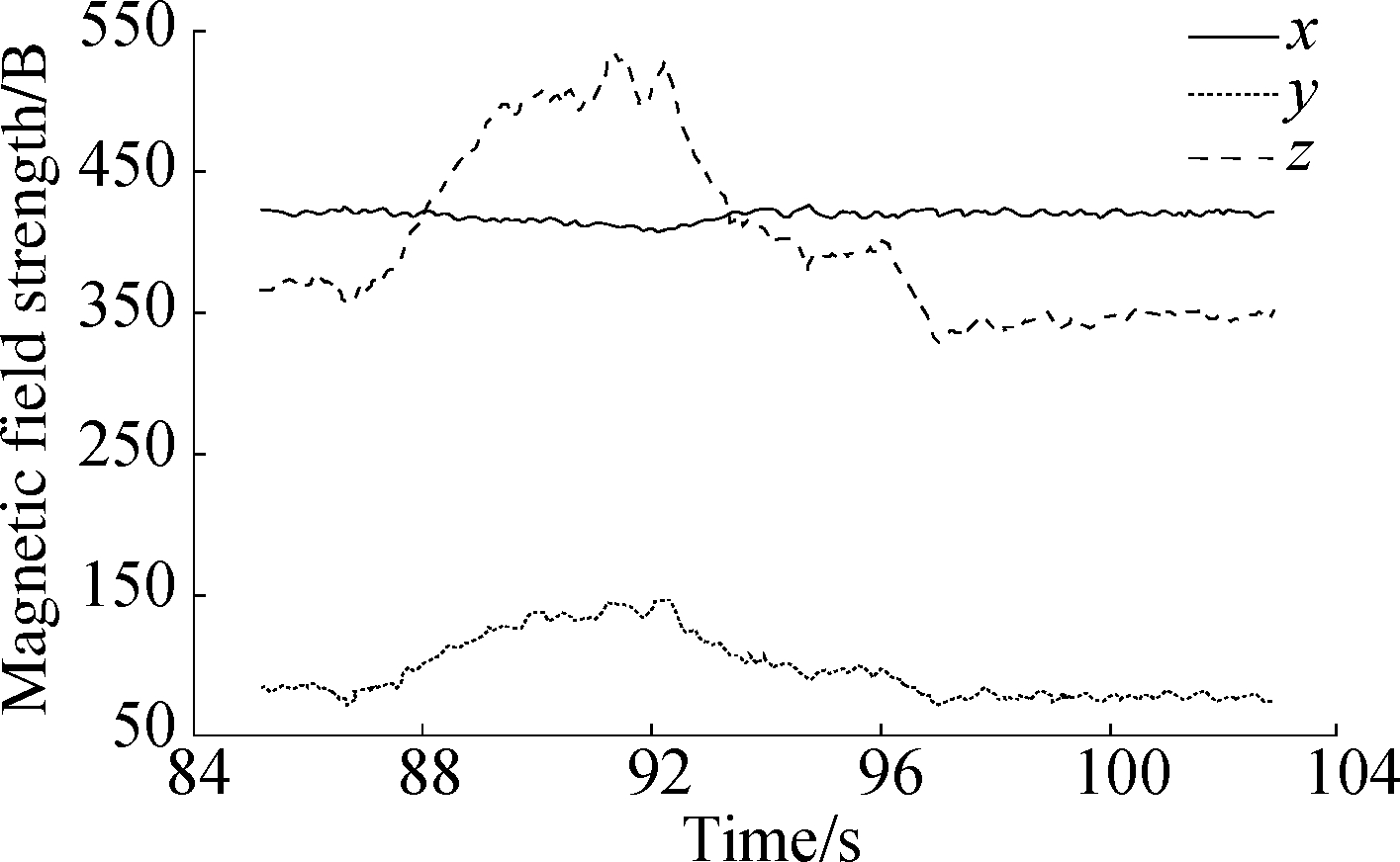
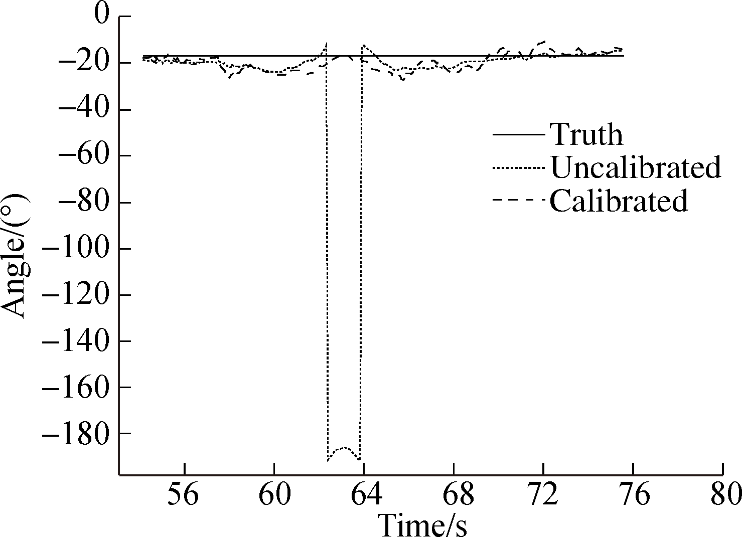
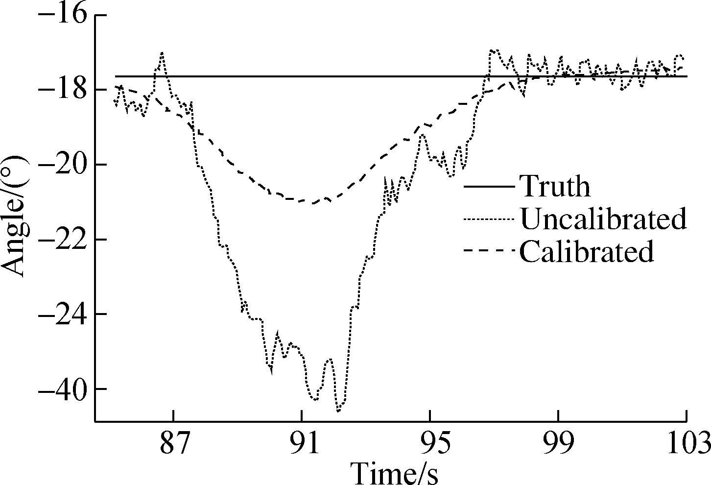
In this work, an approach to the dynamic calculation and correction of the heading angle is proposed. The effect of this approach under different interference intensities is verified by experiments. For the ease of comparison of the test results, we fix the steering gear so as to obtain a fixed angle under the condition in which the carrier is driven straight and need not to be turned. The data of the three-axis magnetometer in Path B are shown in Fig. 4. The heading angles under Paths A and B are presented in Fig. 5. Path A is closer to the interference source than Path B and is thus prone to stronger interference intensity. A serious deviation of the uncalibrated heading angle appears near the strong interference in Fig. 5 (a), and the deviation of the uncalibrated heading angle is minimal. Meanwhile, the calibrated value restores the true heading angle more closely in Fig. 5 (a) than in Fig. 5 (b).
The mean values of the uncalibrated heading angle error and calibrated heading angle error are 13.450 2° and 2.127 8°, respectively. The STD values of the uncalibrated heading angle error and calibrated heading angle error are 42.970 5° and 3.727 6°, respectively. The accuracy improves by about 60% after calibration. The mean values of the uncalibrated heading angle error and calibrated heading angle error are 2.467 0° and 1.220 7°, respectively. The STD values of the uncalibrated heading angle error and calibrated heading angle error are 2.981 2° and 1.226 7°, respectively. The accuracy improves by about 50% after calibration.
(a)
(b)
Fig.4 Output of triaxial magnetometer.(a) Large interference; (b) Small interference
(a)
(b)
Fig.5 Heading angle.(a) Path A; (b) Path B
2.2 Results for fusion based on different weight factors p
The experimental data are generated by random movement in the building. To facilitate the comparison, we preset the carrier trajectory in the experimental site and obtain the true heading angle on the basis of the carrier movement along the trajectory. After data elimination, 10 000 valid data are finally selected. Each set of experimental data includes the observation value of the magnetometer at the previous time, the angular velocity increment of the gyroscope at the current time, the observation value of the magnetometer at the current time, and the real angle at the current time. The sum of the previous magnetometer value, current angular velocity increment, and current magnetometer value are used as the input of the RF algorithm. Then, p is calculated by Eq.(22) as the output for the training model. Finally, the trained model is obtained. In the actual operation, we set the sampling time to 0.1 s. Thus, the p value is adjusted every 0.1 s.
Fig 6. compares the results of the fusion algorithm using fixed p-values and those based on RF prediction. The weight factor p affects the value of the final heading angle. The value is biased toward the gyroscope as p increases. The mean values of the heading angles are 2.2°,-1.72°, and 5.7° when the three coefficients correspond to eastward straight movement. The heading angles are 90.88°, 92.29°, and 87.25° when sensors are traveling northward. The heading angle corresponding to the straight line in the east should be 0, and the heading angle to the north should be 90°. Thus, when the weight factor p is calculated by the RF algorithm, the heading angle average is relatively close to the actual value. The heading angle variances of the three coefficients are 1.86°, 40.07°, and 11.87°. Therefore, relative to a fixed p-value, when the weight factor p is calculated by the RF algorithm, the calculated weighted heading angle is relatively stable.
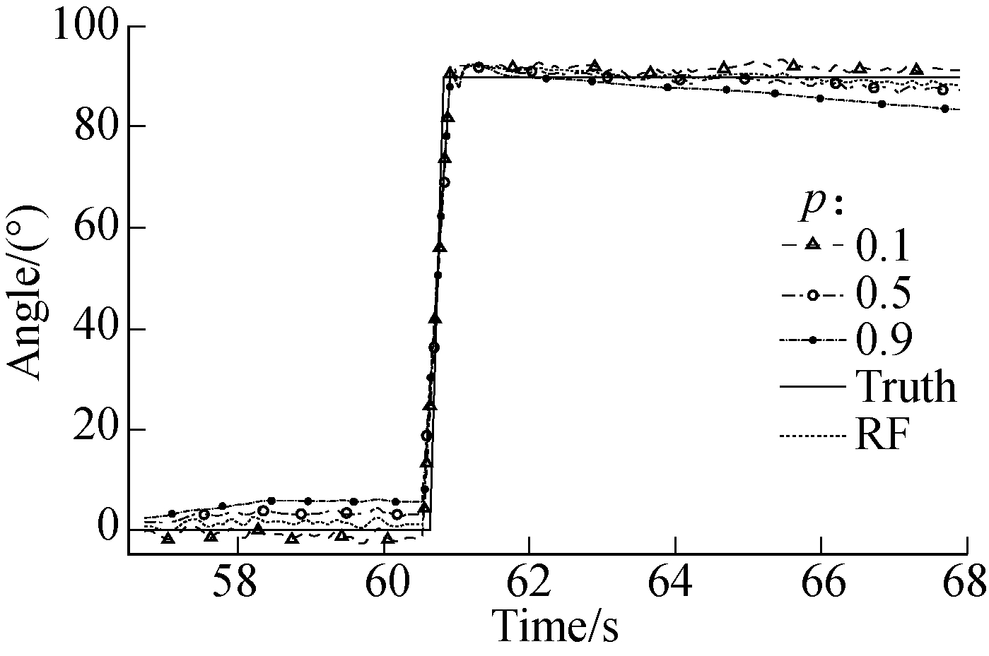
Fig.6 Fusion results for different weight factors p
2.3 Results for fusion based on IMU and magnetometer
In the proposed weighted fusion approach, the gyroscope output value collected in real time is used as the increment of the heading angle calculated at the last moment to predict a heading angle. Then, the predicted heading angle and magnetometer output collected in real time are used as the input of the RF model to obtain the weight factor p. Finally, the current heading angle is calculated by p and the predicted heading angle and magnetometer output value collected in real time. In the experiment, the heading angle is determined by the proposed weighted fusion approach. The comparison experiment is shown in Fig.7.
Fig. 7 shows the heading angles corresponding to the magnetometer, gyroscope, and weighted fusion approach during the left turn. As the gyroscope measures the rota-tion angle, the current direction is equal to the direction of the previous time plus the rotation angle. Thus, the change is relatively stable. The magnetometer directly measures the absolute direction, and the measured heading angle changes relatively steeply even if filtering is performed. As shown in Fig. 7, both sensors can be sensitive to changes in the sensed direction. The magnetometer and gyroscope can effectively describe the trend of a user’s motion direction. The weighted fusion approach combines the advantages of the two sensors and ensures that the final heading angle is relatively accurate and stable.

Fig.7 Heading angle of different sensors
3 Conclusions
1) A dynamic error model of a magnetometer is set up on the basis of error classification in magnetometer measurement. This model can reduce the measurement error of the magnetometer.
2) An approach that entails dynamically calculating the heading angle is presented. This approach promotes the accuracy of magnetic heading calculation through sensor fusion. In the weighted fusion approach, the weight factor p is calculated using the RF algorithm. Then, the heading angle is calculated by p. The weight factor p determines whether the heading angle is biased toward the magnetometer or the gyroscope.
3)The experimental results show that the proposed approach improves calculation accuracy by about 60%. The proposed approach can also reduce magnetic field interference, but it cannot eliminate it completely.
[1]Patonis P, Patias P, Tziavos I, et al. A fusion approach for combining low-cost IMU/magnetometer outputs for use in applications on mobile devices[J]. Sensors, 2017, 18(8):2616-2632. DOI: 10. 3390/s18082616.
[2]Cong L, Li E C, Qin H L, et al. A performance improvement method for low-cost land vehicle GPS/MEMS-INS attitude determination[J].Sensors (Basel, Switzerland), 2015, 15(3): 5722-5746. DOI:10.3390/s150305722.
[3]Hellmers H, Kasmi Z, Norrdine A, et al. Accurate 3D positioning for a mobile platform in non-line-of-sight scenarios based on IMU/magnetometer sensor fusion[J]. Sensors, 2018, 18(1): 126-144. DOI:10. 3390/s18010126.
[4]Zhai Y J, Zhao H L, Zhao M. Design of electric patrol UAVs based on a dual antenna system[J]. Energies, 2018, 11(4): 866-873. DOI:10.3390/en11040866.
[5]Ambati P R, Padhi R. Robust auto-landing of fixed-wing UAVs using neuro-adaptive design[J]. Control Engineering Practice, 2017, 60: 218-232. DOI:10.1016/j.conengprac.2016.03.017.
[6]Rosario M, Khamis H, Ngo P, et al. Computationally efficient adaptive error-state Kalman filter for attitude estimation[J]. IEEE Sensors Journal, 2018, 18(22): 9332-9342. DIO 10.1109/jsen.2018.2864989.
[7]Yin G, Zhang L. Magnetic heading compensation approach based on magnetic interferential signal inversion[J]. Sensors and Actuators A: Physical, 2018, 275:1-10. DOI: 10.1016/j.sna.2018.03.043.
[8]Wang Q, Yin J, Noureldin A. Research on an improved approach for foot-mounted inertial/magnetometer pedestrian-positioning based on the adaptive gradient descent algorithm[J]. Sensors, 2018, 18(12):4105-4122. DOI:10.3390/s18124105.
[9]Xing H F, Chen Z Y, Yang H T, et al. Self-alignment MEMS IMU approach based on the rotation modulation technique on a swing base[J]. Sensors, 2018, 18(4): 1178-1199. DOI: 10.3390/s18041178.
[10]Bao G Z, Wickenbrock A, Rochester S, et al. Suppression of the nonlinear Zeeman effect and heading error in earth-field-range alkali-vapor magnetometers[J]. Physical Review Letters, 2018, 120(3): 033202. DOI:10.1103/PhysRevLett.120.033202.
[11]Li G Z, Zhao S, Zhu R. Wearable anemometer with multi-sensing of wind absolute orientation, wind speed, attitude, and heading[J]. IEEE Sensors Journal, 2019, 19(1):297-303. DOI 10.1109/JSEN.2018.2874809.
[12]Song X, Li X, Tang W C, et al. A fusion strategy for reliable vehicle positioning utilizing RFID and in-vehicle sensors[J]. Information Fusion, 2016, 31(31): 76-86. DOI 10.1016/j.inffus.2016.01.003.
[13]Rantanen J, Ruotsalainen L, Kirkkojaakkola M, et al. Height measurement in seamless indoor/outdoor infrastructure-free navigation[J]. IEEE Transactions on Instrumentation and Measuremen, 2019, 68(4): 1199-1209.DOI 10.1109/TIM.2018.2863978.
[14]Xu Q, Li X, Li B. A reliable hybrid positioning methodology for land vehicles using low-cost sensors[J]. IEEE Transactions on Intelligent Transportation System, 2016, 17(3):834-847. DOI:10.1109/TITS.2015.2487518.
[15]Wu J, Zhou Z, Fourati H, et al. A super fast attitude determination algorithm for consumer-level accelerometer and magnetometer[J]. IEEE Transactions on Consumer Electronics, 2018, 64(3): 375-381. DOI 10.1109/TCE.2018.2859625.
[16]Li X, Chen W, Chan C. A reliable multisensor fusion strategy for land vehicle positioning using low-cost sensors[J]. Proceedings of the Institution of Mechanical Engineers, Part D: Journal of Automobile Engineering, 2014, 228(12): 1375-1397. DOI 10.1177/0954407014533518.
[17]Vochin M, Vulpe A, Boicescu L, et al. An intelligent low-power displaying system with integrated emergency alerting capability[J]. Sensors, 2019, 19(3): 666. DOI 10.3390/s19030666.
[18]Qin H L, Cong L, Sun X L. Accuracy improvement of GPS/MEMS-INS integrated navigation system during GPS signal outage for land vehicle navigation[J]. Journal of Systems Engineering and Electronics, 2012, 23(2): 256-264. DOI 10.1109/JSEE.2012.00033.
[19]Jiang C, Zhang S B, Zhang Q Z. Adaptive estimation of multiple fading factors for GPS/INS integrated navigation systems[J]. Sensors, 2017, 17(6): 1254-1271. DOI 10.3390/s17061254.
[20]Cho S Y, Kim B D. Adaptive IIR/FIR fusion filter and its application to the INS/GPS integrated system[J]. Automatica, 2008, 44(8): 2040-2047. DOI 10.1016/j.automatica.2007.11.009.
[21]Pasku V, Angelis A D, Angelis G D, et al. Magnetic field-based positioning systems[J]. IEEE Communications Surveys and Tutorials, 2017, 19(3):2003-2017. DOI 10.1109/COMST.2017.2684087.