With the development of advanced sensing and artificial intelligence techniques, autonomous vehicles are gaining increasing attention from the industry and academic communities and are regarded as the most promising industry for improving road safety in the future [1-3].An autonomous vehicle is a highly integrated electromechanical coupling system comprising many vital technologies, such as car perception, image identification and processing, trajectory planning, trajectory following control, anti-lock brake, active suspension control technology, and automatic parking technologies.Trajectory following control, in particular, plays a vital role in the driving performances of autonomous vehicles.This technology is mainly aimed at tracking desired trajectories continuously and smoothly with the highest precision possible.
In the past decades, many studies have focused on trajectory following for autonomous vehicles.Specifically, these studies have mainly applied advanced control algorithms or proposed novel control algorithms so as to ensure driving safety and thereby achieve good control in situations in which vehicle models cannot be established accurately and uncertain external disturbances exist.At present, the control algorithms that are widely used in trajectory following control for autonomous vehicles include feedback linearization[4-5], sliding mode control[6-10], neural network control [11-13], and model predictive control [14-19].
Although a large number of studies in trajectory following for autonomous vehicles have been carried out, certain shortcomings remain.Most existing studies aimed to propose or use a new method from the control algorithm itself to show its outstanding performance by comparing it with other control methods.Only a few articles report calculation methods for trajectory following control that are detailed and complete, especially in terms of the calculation of errors, determination of tracking points, and design of feedforward controllers.For example, the work in Refs.[20-23]did not consider feedforward control in eliminating steady-state errors.Hence, the results are not useful in evaluating and fairly comparing the performance of control methods.
Accordingly,the current study presents a complete calculation method for trajectory following control for autonomous vehicles by calculating real-time tracking points on the basis of current vehicle states.The proposed method’s implementation steps, in which computational equations are deduced by the dynamic equation of the global coordinate and control equation of trajectory following with an error form, are introduced systematically.A sample simulation of trajectory following control based on a linear quadratic regulator(LQR)with a feedforward controller is performed by developing a program in MATLAB to facilitate the understanding of the calculation method.The implementation process and simulation results are described accordingly.Computational cost and reliability analyses are also performed.
1 Vehicle Dynamical Modeling for Trajectory Following Control
The vehicle handling dynamics model using three degrees of freedom(DOF)essentially describes trajectory following control.To facilitate the description of the calculation method for trajectory following control, this work makes the following main assumptions: 1)The differences in the tire cornering properties between the left and right wheels due to load variation are ignored, and the tire model is approximated as linear; 2)The vehicle only executes front-wheel steering; 3)Longitudinal velocity is a constant value.The vehicle dynamical model is shown in Fig.1, where OXYZ represents the global coordinate system and Cxyz represents the vehicle coordinate system whose origin is the vehicle centroid and the x-axis is the driving direction.
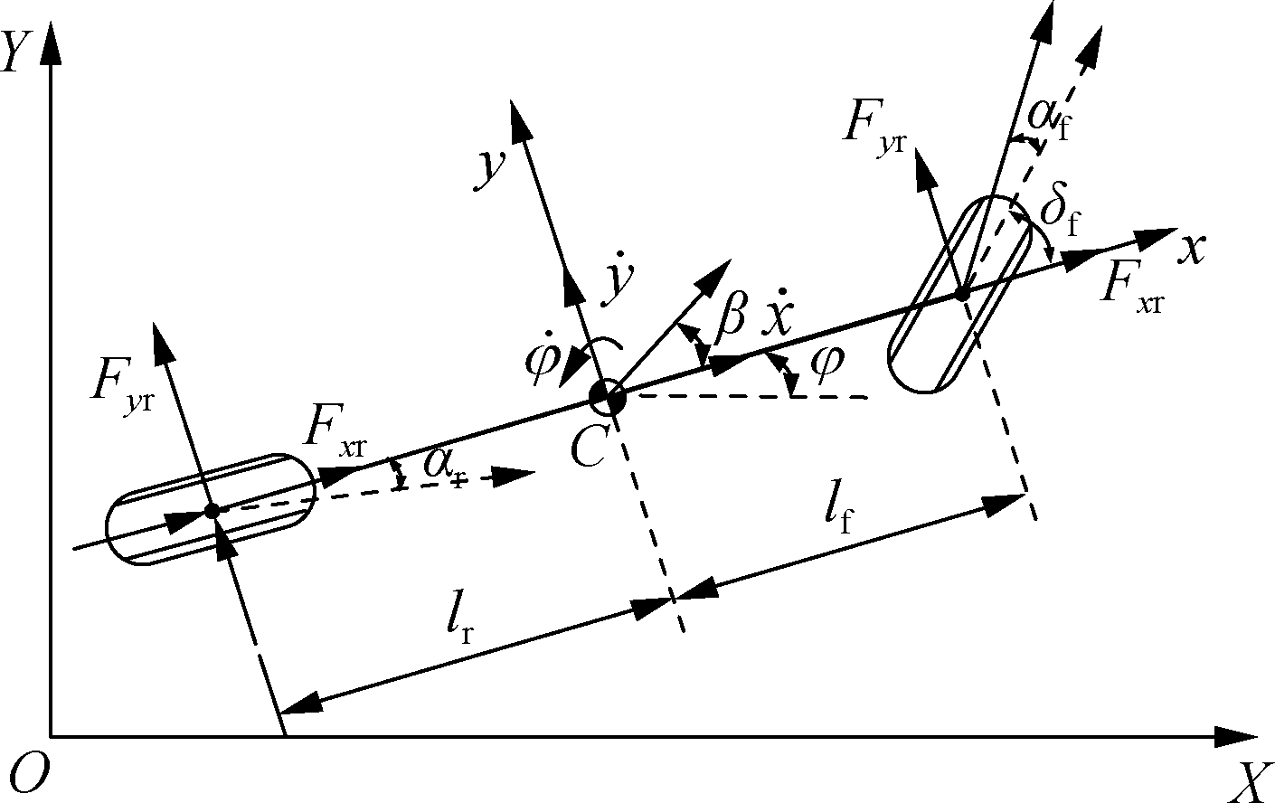
Fig.1 Vehicle dynamical model
1.1 Dynamical equation under the vehicle coordinate system
In the maneuvering dynamical model, the external force transmitted by the tire to the vehicle primarily depends on the speed variable rather than on the absolute position coordinates and heading angle of the vehicle.Therefore, the dynamical equation is established using the coordinate system Cxyz fixed on the vehicle.According to the assumption that the longitudinal velocity is constant, the dynamical equation can be obtained as [8,16]
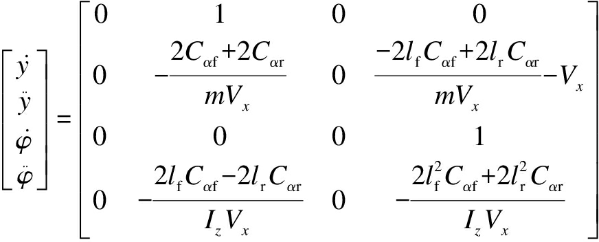 ·
·
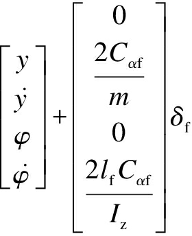
(1)
where y is the lateral displacement; ![]() is the yaw rate; m is the total vehicle mass; Iz represents the vehicle inertia around the axis Cz; Vx is the longitudinal velocity; δf is the front steering angle; lf and lr denote the distances between the front and rear wheel axles with C, respectively; and Cαf and Cαr represent the front and rear cornering stiffness, respectively.
is the yaw rate; m is the total vehicle mass; Iz represents the vehicle inertia around the axis Cz; Vx is the longitudinal velocity; δf is the front steering angle; lf and lr denote the distances between the front and rear wheel axles with C, respectively; and Cαf and Cαr represent the front and rear cornering stiffness, respectively.
1.2 Dynamical equation under the global coordinate system
When performing trajectory following control in an actual road, an autonomous vehicle needs to accurately measure and estimate the current vehicle states, such as the yaw rate, longitudinal velocity, and lateral velocity, by utilizing a GPS/INS navigation system [21].Similarly, an autonomous vehicle needs to obtain these states by using the dynamical equation on the global coordinate system when performing simulation control for trajectory following.An increasing number of studies have adopted the multibody dynamical model on the basis of dynamic software, such as ADAMS, SIMPACK, and CarSim, to compute vehicle states accurately.
As the current work mainly focuses on the calculation method for trajectory following, a 3-DOF dynamical model is employed for computing vehicle states.According to the momentum and moment of momentum theorem under the assumption of constant longitudinal velocity, the dynamical equation on the global coordinate system can be obtained as
(2)
(3)
(4)
where X and Y represent the vehicle’s center-of-mass coordinate with respect to OXYZ; φ represents the attitude of oxyz with respect to OXYZ(i.e., yaw angle of the vehicle); and Fyf and Fyr denote the y-axis component of the front and rear lateral tire forces with respect to oxyz, respectively.
The transformation relationship between oxyz and OXYZ is given by
(5)
Fyf and Fyr are respectively calculated by the tire side-slip characteristics as
(6)
(7)
The dynamical equations under the global coordinate system can be obtained by substituting Eqs.(5)to(7)into Eqs.(2)to(4).
1.3 Control equation with error form
The vehicle trajectory following model is shown in Fig.2, where Cd is the desired position and C is the real position of the vehicle’s center of mass.In Fig.2, point Cd is on the desired trajectory, and vector CCd and the tangent of Cd are perpendicular.The desired coordinate system Cdxdydzd can be defined as follows: the tangent of Cd is the x-axis, and vector CdC is the y-axis.In Fig.2, φdes and ![]() respectively represent the desired yaw angle and yaw rate of the vehicle; Vxdes represents the desired longitudinal velocity; and Vx,
respectively represent the desired yaw angle and yaw rate of the vehicle; Vxdes represents the desired longitudinal velocity; and Vx, ![]() respectively denote the actual longitudinal velocity, lateral velocity, lateral acceleration, yaw angle, yaw rate, and angular acceleration of the vehicle.The magnitudes of Vxdes and Vx are equal, but their directions are different.
respectively denote the actual longitudinal velocity, lateral velocity, lateral acceleration, yaw angle, yaw rate, and angular acceleration of the vehicle.The magnitudes of Vxdes and Vx are equal, but their directions are different.
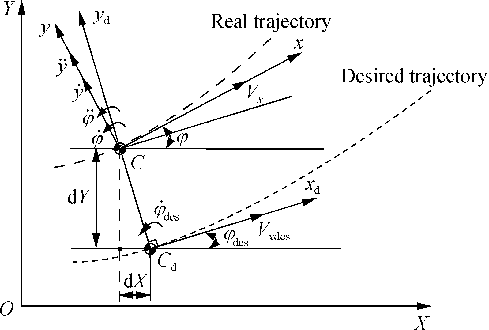
Fig.2 Trajectory following model
Transforming the states into the same coordinate system is necessary to obtain the errors between actual states and desired states.After performing the projection operation of the states into the desired coordinate system, the error between the actual and desired lateral accelerations can be expressed as
(8)
The error between the actual lateral and the desired lateral velocities is given by
(9)
As the value of φ-φdes is extremely small, ![]() is far less than Vx, and the magnitudes of Vx and Vdes are equal.Therefore, Eqs.(8)and(9)can be simplified as
is far less than Vx, and the magnitudes of Vx and Vdes are equal.Therefore, Eqs.(8)and(9)can be simplified as
(10)
(11)
The error between the actual and desired yaw angles is defined as
eφ=φ-φdes
(12)
The error between the actual yaw rate and the desired yaw rate is given as
(13)
By substituting Eqs.(10)to(13)into Eq.(1), the dynamical equation with the error form can be obtained as
(14)
where


2 Calculation Method for Trajectory Following Control
With a plan for the desired trajectory in place, trajectory following control is aimed toward driving the vehicle along such trajectory as closely as possible.Control algorithms include PID control, LQR control, sliding mode control, and fuzzy neural network control.In the current work, the LQR method, which is one of the most representative control methods, is adopted to facilitate the understanding of the calculation method for trajectory following control.
To realize trajectory following control,this study proposes the following six steps:
Step 1 Plan the desired trajectory according to the driving purpose.
Step 2 Obtain the current vehicle states, such as actual position, longitudinal velocity, lateral velocity, yaw angle, and yaw rate, on the basis of the vehicle dynamical model or vehicle perception equipment.
Step 3 Determine the desired point states and their deviations between the actual point and the tracking point according to the current vehicle states and the desired trajectory.
Step 4 Calculate the control input on the basis of the control equation with the error form, feedforward control, and LQR control method.
Step 5 Obtain the actual vehicle position, longitudinal velocity, lateral velocity, yaw angle, and yaw rate at the next moment by using the vehicle simulation model after inputting the control quantity obtained from step 4.
Step 6 Repeat steps 2 to 5 until the end.
2.1 Planning the desired trajectory
Several geometric forms can be used to plan the following trajectory.In particular, polynomial trajectories are the most common form used in automated driving [24-26].In this work, the following cubic polynomial is adopted to express the desired trajectory:
Y=f(X)=a3X3+a2X2+a1X1+a0
(15)
where a0 to a3 are the fit coefficients of the cubic polynomial.
2.2 Calculating errors between desired and actual states
The assumption is that vehicle states ![]() at moment t have been obtained on the basis of the vehicle dynamical model.The following five calculation steps are given for calculating the desired states and actual errors at moment t:
at moment t have been obtained on the basis of the vehicle dynamical model.The following five calculation steps are given for calculating the desired states and actual errors at moment t:
1)Calculate Xdes(t)and Ydes(t).According to the actual point C[X(t),Y(t)]from the vehicle’s center of mass, calculate tracking point Cd with trajectory function y=f(x).The straight line CCd and tangent of Cd satisfy
(Y(t)-f(Xdes(t)))f′(Xdes(t))+X(t)-Xdes(t)=0
(16)
Xdes(t)can be easily obtained by solving the algebraic Eq.(16)while considering X(t)as the initial point.Then, Ydes(t)can be acquired by trajectory function y=f(x).
2)Calculate φdes(t).In accordance with Xdes(t)and trajectory function y=f(x), φdes(t)is given as
φdes(t)=arctanf(Xdes(t))
(17)
3)Determine ![]() With the curvature radius formula, the curvature of point Cd is given as
With the curvature radius formula, the curvature of point Cd is given as
(18)
Then, the desired yaw rate at moment t is calculated as
(19)
4)Calculate ey(t)and ![]() By transforming the actual and desired points into the desired coordinate system Cdxdydzd, ey(t)and
By transforming the actual and desired points into the desired coordinate system Cdxdydzd, ey(t)and ![]() can be respectively calculated as
can be respectively calculated as
ey(t)=-(X(t)-Xdes(t))sin(φdes(t))+
(Y(t)-Ydes(t))cos(φdes(t))
(20)
(21)
5)Obtain eφ(t)and ![]() according to Eqs.(12)and(13).
according to Eqs.(12)and(13).
2.3 Determining the control input
According to Eq.(14)and the LQR method, the control input δf1(t)is obtained as
(22)
where K is the feedback gain matrix of the optimal control and can be expressed as
K=R-1BTP
(23)
where P can be obtained by the Riccati equation, which has the following form:
PA+ATP-PBR-1BTP+Q=0
(24)
where R is the weight matrix on the control input and Q is the weight matrix on the error.
As the variation of the desired angular velocity results from the different curvatures of the desired trajectory at different times, a feedforward controller is adopted to minimize tracking errors and ensure zero steady-state errors.The autonomous vehicle with only front wheel steering belongs to the under-actuated control system, which cannot completely eliminate the steady-state errors from the two states.Nevertheless, we can ensure zero lateral steady-state error, which is more important than angular steady-state error.
Therefore, the feedforward controller—used for completely eliminating the lateral steady-state error—is introduced in detail.However, an angular steady-state error still exists in the under-actuated control system.According to feedback gain matrix K, the closed-loop matrix Ab can be expressed as
Ab=A-BK
(25)
As the first and third rows of B are zero, Ab is always satisfied as follows, regardless of the value of K:
Ab(1,1)=Ab(1,3)=Ab(1,4)=0, Ab(1,2)=1
(26)
Ab(3,1)=Ab(3,2)=Ab(3,3)=0, Ab(3,4)=1
(27)
Hence, on the basis of Eq.(14)and ![]() the relationship between the steady-state error and the feedforward control can be written as the following matrix equation:
the relationship between the steady-state error and the feedforward control can be written as the following matrix equation:
(28)
where eys(t)and eφs(t)respectively denote the lateral and angular steady-state errors at moment t.
After ensuring eys(t)= 0, the steady-state angular error and feedforward control quantity at moment t can be expressed as the following matrix equation:
(29)
By combining the LQR with the feedforward control, the total control input can be calculated as
δf(t)=δf1(t)+δf2(t)
(30)
As a result of the demand for vehicle safety and physical implementation, the control input is not completely determined by Eq.(30), and the value range needs to be considered.Herein, the ranges of the front steering angle and front steering angle velocity are respectively given by
δmin≤δf(t)≤δmax
(31)
(32)
where δmin and δmax represent the maximum and minimum values of the front steering angle, respectively; and ![]() represent the maximum and minimum values of the front steering angle velocity, respectively.
represent the maximum and minimum values of the front steering angle velocity, respectively.
2.4 Vehicle dynamics simulation under control input
The next moment vehicle ![]() be calculated according to the vehicle dynamical model in Section 1.2 and the control input obtained by Section 2.3.By repeating the steps detailed in Sections 2.2, 2.3, and 2.4 until the end, the simulation results for trajectory following control can be obtained.
be calculated according to the vehicle dynamical model in Section 1.2 and the control input obtained by Section 2.3.By repeating the steps detailed in Sections 2.2, 2.3, and 2.4 until the end, the simulation results for trajectory following control can be obtained.
3 Simulation and Analysis
A program is independently developed in MATLAB to evaluate the feasibility and effectiveness of the proposed calculation method in Section 2.The developed program is used to implement the trajectory following control simulation.
3.1 Desired trajectory
The desired trajectory adopts the polynomial expression where a0=0, a1=0.999 886 710 218 506, a2=-0.004 998 300 653 278, and a3=-0.566 448 9×10⁻⁸, as shown in Fig.3.The desired trajectory has a minimum curvature radius of 100 mm.The control effect of trajectory following is known to depend largely on the curvature radius of the desired trajectory.In other words, the smaller the curvature radius is, the harder the control becomes.Following this trajectory under the longitudinal velocity of 10 m/s is relatively difficult, but this trajectory has certain representativeness.

Fig.3 Desired trajectory curve
3.2 Vehicle simulation parameters
The simulation parameters are shown in Tab.1.
Tab.1 Simulation parameters of the vehicle model

ParameterValueVehicle mass m/kg 1 575Vehicle yaw moment Iz/(kg·m2 2 875Front-CG distance lf/m 1.2Rear-CG distance lr/m1.6Cornering stiffness of front tires Cf/ kN·rad-1 19Cornering stiffness of rear tires Cr/ kN·rad-1 33Maximum steering angle δmax/rad0.523 6Minimum steering angle δmin/rad-0.523 6 Maximum steering angle velocity δ max/ rad·s-1 0.261 8Minimum steering angle velocity δ min/ rad·s-1 -0.261 8 Longitudinal velocity Vx/ m·s-1 10
3.3 Simulation results and analysis
The initial states are defined as follows: The yaw angle of the vehicle relative to the global coordinate system is 0.785 3 rad, the yaw rate is 0 rad/s, the longitudinal velocity is 10 m/s, and the lateral velocity is 0 m/s.The global coordinate of the vehicle’s center of mass is(0, 1)m.In the initial states, the simulation time is set to 30 s, and the simulation results of the trajectory following control are shown in Figs.4 to 6.
Fig.4 shows the tracking process from the actual vehicle position to the desired trajectory position.The simulation presents a good trajectory following effect, and the actual vehicle position fluctuates around the desired trajectory at a small-scale level.The standard deviation between the actual trajectory and the desired trajectory is calculated as 0.11 m.
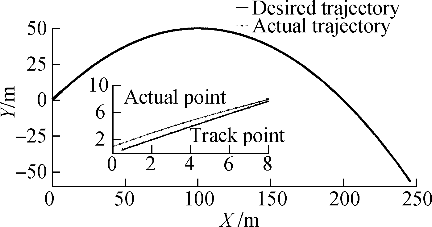
Fig.4 Contrast between desired and actual trajectories
Fig.5 presents the error responses.The lateral and angular errors gradually decrease by controlling the front steering angle, which achieves the desired control effect.Furthermore, the steady-state errors gradually tend to approach zero because of the introduction of feedforward control.As illustrated in Fig.5(a), the lateral steady-state error can be completely eliminated, although the trajectory curvature is not zero.The simulation results also reveal that when the vehicle passes through the position with a relatively large curvature, the tracking effect deteriorates to a certain extent despite the introduction of feedforward control.

(a)

(b)
Fig.5 Response of error.(a)Lateral error;(b)Angular error
Fig.6 shows the response of the front steering angle provided by the LQR controller with feedforward control.The front steering angle is limited to the given range, which meets the requirements of the vehicle’s physical realizability.In addition, the front steering angle is much smaller than the given boundary value, and the variation range of the angle is small.These features can strongly guarantee vehicle safety.

Fig.6 Response of front steering angle
For the purpose of illustrating the strong anti-interference ability of the proposed method that calculates trace points in real-time on the basis of current vehicle states, an accidental interference in 7.5 s is assumed to cause large deviations(0.5 m, 0.5 m, 0.1 rad)between the actual vehicle position and the calculated position.Figs.7 and 8 show the responses of the error and front steering angle.After being greatly disturbed in 7.5 s, the system automatically adjusts the trace point to eliminate the deviation according to the current actual states so that the vehicle drives along the desired trajectory and achieves a good control effect.

(a)

(b)
Fig.7 Response of error with accidental interference.(a)Lateral error;(b)Angular error
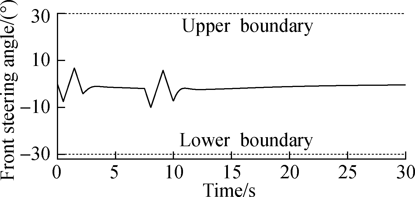
Fig.8 Response of front steering angle with accidental interference
3.4 Computational cost
Computational cost is a crucial factor that determines whether the proposed algorithm can be used in practice.Hence, it requires evaluation.The computer configurations for the simulation are as follows: Windows 10 64-bit operating system, AMD Ryzen 7 CPU, 16 GB RAM with 3 200 MHz, and MATLAB version R2018a.
Under this computing environment, the computation time can be obtained by using a timer.When the simulation time is set to 30 s, the computation time is 0.56 s, which is the average time for 20 repetitions.Furthermore, the timer indicates that the computational cost mainly depends on “fsolve”[i.e., the solution of algebraic Eq.(16)].Nevertheless, the computation time is so small that the real-time performance is generally easy to satisfy under the computing environment.The algorithm can be further optimized in the future, particularly in terms of the calculation of the tracking point.
4 Reliability Analysis and Discussion by Experimental Comparison
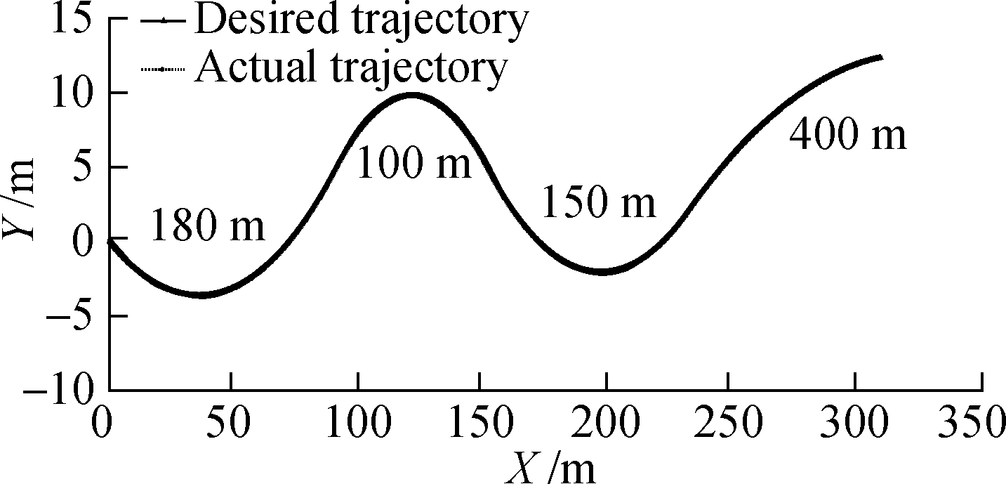
The simulation results based on the proposed calculation method and the experimental results from Ref.[21]are compared under the same vehicle parameters and tracking trajectory to further analyze the reliability of the simulation results.The tracking trajectory is defined as trajectory 1.The simulation parameters of the experimental vehicle are not given in the literature, but after a careful search [12], the vehicle parameters are established.Meanwhile, Gaussian noise considering sensor accuracy is added to the vehicle state in the simulation to effectively reflect the actual states of the vehicle.The coordinate axis and its range are unified to ensure a good comparison with the results from the literature(see Figs.9 to 12).
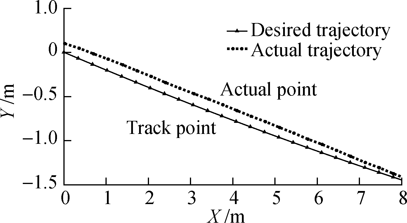
For clarity, an enlarged view at 0-8 m is shown in Fig.9(b).Fig.9 shows that good tracking performance is achieved.
(a)
(b)
Fig.9 Desired trajectory and actual trajectory based on trajectory 1.(a)Global view at 0 to 320 m;(b)Partial enlarged view at 0 to 8 m
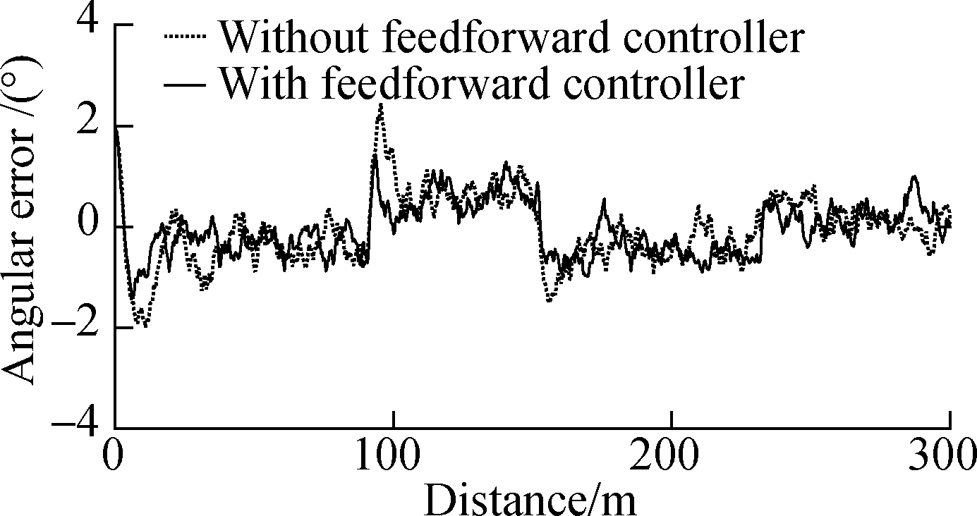
Feedforward control is not considered in eliminating the steady-state error in this study.The dotted curves in Figs.10 to 12 show the counterparts without the feedforward controller(i.e., no δf2).Relative to this literature, the simulation results without the feedforward controller(see Figs.10 to 12)are consistent with the experimental results.The simulation results of yaw rate and front steering angle, in particular, are nearly identical to the experi-mental results.Hence, the simulation results are reliable, and the proposed calculation method is feasible.

(a)
(b)
Fig.10 Response of error based on trajectory 1.(a)Lateral error;(b)Angular error

Fig.11 Response of yaw rate based on trajectory 1

Fig.12 Response of front steering angle based on trajectory 1
According to the complete calculation method proposed in this work, the feedforward controller should also be considered to obtain good control performance.The solid curves in Figs.10 to 12 show the simulation results with the feedforward controller.The lateral steady-state error can be adjusted to zero while the changes in the angular error, yaw rate, and front steering angle are not apparent.After careful observation(see Figs.10 to 12), the angular error, yaw rate, and front wheel angle are slightly smaller than their counterparts in the case without the feedforward controller.Hence, a good control effect is achieved with the complete calculation method for trajectory following control despite the control method being traditional.
5 Conclusions
1)A complete calculation method is proposed for the trajectory following control of autonomous vehicles.The implementation steps are also systematically introduced.The feedforward controller with LQR is designed for completely eliminating lateral steady-state errors according to the characteristics of the dynamical equation.
2)A program is independently developed in MATLAB, and a sample simulation is performed.The simulation results show that the control strategies based on the proposed calculation method achieve strong tracking and anti-interference performance.
3)The simulation results are determined to be reliable, and the proposed calculation method is deemed feasible by comparing the experimental results from the literature.In addition, good control performance is achieved with the proposed complete calculation method for trajectory following control, particularly through the introduction of the feedforward controller.
[1] Luo Y G, Xiang Y, Cao K, et al.A dynamic automated lane change maneuver based on vehicle-to-vehicle communication[J].Transportation Research Part C: Emerging Technologies, 2016, 62: 87-102.DOI:10.1016/j.trc.2015.11.011.
[2] Li X H, Sun Z P, Cao D P, et al.Development of a new integrated local trajectory planning and tracking control framework for autonomous ground vehicles[J].Mechanical Systems and Signal Processing, 2017, 87: 118-137.DOI:10.1016/j.ymssp.2015.10.021.
[3] Amer N H, Zamzuri H, Hudha K, et al.Modelling and control strategies in path tracking control for autonomous ground vehicles: A review of state of the art and challenges[J].Journal of Intelligent & Robotic Systems, 2017, 86(2): 225-254.DOI:10.1007/s10846-016-0442-0.
[4] Javid S, Eghtesad M, Khayatian A, et al.Experimental study of dynamic based feedback linearization for trajectory tracking of a four-wheel autonomous ground vehicle[J].Autonomous Robots, 2005, 19(1): 27-40.DOI:10.1007/s10514-005-0604-6.
[5] Dekker L G, Marshall J A, Larsson J.Experiments in feedback linearized iterative learning-based path following for center-articulated industrial vehicles[J].Journal of Field Robotics, 2019, 36(5): 955-972.DOI:10.1002/rob.21864.
[6] Taghia J, Wang X, Lam S, et al.A sliding mode controller with a nonlinear disturbance observer for a farm vehicle operating in the presence of wheel slip[J].Autonomous Robots, 2017, 41(1): 71-88.DOI:10.1007/s10514-015-9530-4.
[7] Hu C, Wang R R, Yan F J.Integral sliding mode-based composite nonlinear feedback control for path following of four-wheel independently actuated autonomous vehicles[J].IEEE Transactions on Transportation Electrification, 2016, 2(2): 221-230.DOI:10.1109/TTE.2016.2537046.
[8] Xu L H, Wang Y Z, Sun H B, et al.Integrated longitudinal and lateral control for kuafu-Ⅱ autonomous vehicle[J].IEEE Transactions on Intelligent Transportation Systems, 2016, 17(7): 2032-2041.DOI:10.1109/TITS.2015.2498170.
[9] Kayacan E, Kayacan E, Ramon H, et al.Towards agrobots: Trajectory control of an autonomous tractor using type-2 fuzzy logic controllers[J].IEEE/ASME Transactions on Mechatronics, 2015, 20(1): 287-298.DOI:10.1109/TMECH.2013.2291874.
[10] Chebly A, Talj R, Charara A.Coupled longitudinal/lateral controllers for autonomous vehicles navigation, with experimental validation[J].Control Engineering Practice, 2019, 88: 79-96.DOI:10.1016/j.conengprac.2019.05.001.
[11] Han G N, Fu W P, Wang W, et al.The lateral tracking control for the intelligent vehicle based on adaptive PID neural network[J].Sensors(Basel, Switzerland), 2017, 17(6): E1244.DOI:10.3390/s17061244.
[12] Guo J H, Luo Y G, Li K Q.Adaptive coordinated collision avoidance control of autonomous ground vehicles[J].Proceedings of the Institution of Mechanical Engineers, Part Ⅰ: Journal of Systems and Control Engineering, 2018, 232(9): 1120-1133.DOI:10.1177/0959651818774991.
[13] Chen Y M, Lu C, Chu W B.A cooperative driving strategy based on velocity prediction for connected vehicles with robust path-following control[J].IEEE Internet of Things Journal, 2020, 7(5): 3822-3832.DOI:10.1109/JIOT.2020.2969209.
[14] Luan Z K, Zhang J N, Zhao W Z, et al.Trajectory tracking control of autonomous vehicle with random network delay[J].IEEE Transactions on Vehicular Technology, 2020, 69(8): 8140-8150.DOI:10.1109/TVT.2020.2995408.
[15] Yin G D, Li J H, Jin X J, et al.Integration of motion planning and model-predictive-control-based control system for autonomous electric vehicles[J].Transport, 2015, 30(3): 353-360.DOI:10.3846/16484142.2015.1089322.
[16] Yakub F, Mori Y.Comparative study of autonomous path-following vehicle control via model predictive control and linear quadratic control[J].Proceedings of the Institution of Mechanical Engineers, Part D: Journal of Automobile Engineering, 2015, 229(12): 1695-1714.DOI:10.1177/0954407014566031.
[17] Kayacan E, Ramon H, Saeys W.Robust trajectory tracking error model-based predictive control for unmanned ground vehicles[J].IEEE/ASME Transactions on Mechatronics, 2016, 21(2): 806-814.DOI:10.1109/TMECH.2015.2492984.
[18] Ji J, Khajepour A, Melek W W, et al.Path planning and tracking for vehicle collision avoidance based on model predictive control with multiconstraints[J].IEEE Transactions on Vehicular Technology, 2017, 66(2): 952-964.DOI:10.1109/TVT.2016.2555853.
[19] Hu J J, Xiong S S, Zha J L, et al.Lane detection and trajectory tracking control of autonomous vehicle based on model predictive control[J].International Journal of Automotive Technology, 2020, 21(2): 285-295.DOI:10.1007/s12239-020-0027-6.
[20] Yao T.A model predictive controller with longitudinal speed compensation for autonomous vehicle path tracking[J].Applied Sciences, 2019, 9(22): 4739.DOI:10.3390/app9224739.
[21] Guo J H, Luo Y G, Li K Q.An adaptive hierarchical trajectory following control approach of autonomous four-wheel independent drive electric vehicles[J].IEEE Transactions on Intelligent Transportation Systems, 2018, 19(8): 2482-2492.DOI:10.1109/TITS.2017.2749416.
[22] Guo J H, Li K Q, Luo Y G.Coordinated control of autonomous four wheel drive electric vehicles for platooning and trajectory tracking using a hierarchical architecture[J].Journal of Dynamic Systems, Measurement, and Control, 2015, 137(10): 101001.DOI:10.1115/1.4030720.
[23] Sun C Y, Zhang X, Xi L H, et al.Design of a path-tracking steering controller for autonomous vehicles[J].Energies, 2018, 11(6): 1451.DOI:10.3390/en11061451.
[24] Benloucif A, Nguyen A T, Sentouh C, et al.Cooperative trajectory planning for haptic shared control between driver and automation in highway driving[J].IEEE Transactions on Industrial Electronics, 2019, 66(12): 9846-9857.DOI:10.1109/TIE.2019.2893864.
[25] Nguyen A T,Sentouh C, Popieul J C.Driver-automation cooperative approach for shared steering control under multiple system constraints: Design and experiments[J].IEEE Transactions on Industrial Electronics, 2017, 64(5): 3819-3830.DOI:10.1109/TIE.2016.2645146.
[26] Werling M, Kammel S, Ziegler J, et al.Optimal trajectories for time-critical street scenarios using discretized terminal manifolds[J].The International Journal of Robotics Research, 2012, 31(3): 346-359.DOI:10.1177/0278364911423042.