Long-distance pipeline is an efficient way to transport petroleum and natural gas.The pipeline needs to go through wide areas and experience various types of topographic and geological environments.Moreover, the pipeline will erode gradually due to various corrosive elements in petroleum and gas.Thus, when the operating pressure is greater than the wall’s carrying capacity, the pipeline will rupture and ultimately lead to leakage, environmental pollution, and ecological damage[1].Statistical results indicate that in the petrochemical industry, around 1/4 to 2/3 of the pipeline’s shutdown time was due to corrosion.
In the last decades, research on the evaluation of pipeline’sreliability and remaining useful life(RUL)has attracted much attention[2-3].Among them, the first-order reliability method(FORM), second-order reliability method(SORM), and Monte Carlo simulation(MCS)are the commonly used assessment methods.Mosallam et al.[4] assessed the corroded pipeline’s life, and a probability model was established to characterize the pipeline’s performance and corrosion size.Gong et al.[5] applied FORM to evaluate the reliability of the pipeline with corrosion defects.Nahal et al.[6]proposed an empirical mechanical behavior model to evaluate the pipeline’s structural reliability under different corrosion rates, where the leakage, burst failure mode, and the limit state function(LSF)under different corrosion defects were considered.Bouledroua et al.[7]applied the SORM approach to evaluate the reliability of the corroded pipeline under excessive internal pressure.Hasan et al.[8] adopted MCS and first-order second-moment method to analyze the pipeline’s limit state and failure probability.Leira et al.[9] applied the enhanced MCS method to evaluate the reliability of the pipeline with multiple corrosion defects.Mohamed et al.[10] analyzed the structural reliability of corroded pipelines under different operating pressures, and the influence of the corrosion defects’ size on the pipeline’s failure probability was considered.Tee et al.[11]investigated the correlation between time-varying failure modes(which were caused by corrosion deformation, buckling, and wall thrust)and bending stress, and the failure probability was obtained with MCS.
Besides, international criteria were also used to predict the burst pressure of corroded pipelines, including the modified ASME B31G, DNV RP-F101, and PCORRC[12].Zelmati et al.[13] used the modified ASME B31G to calculate the burst pressure of the pipeline.To calculate the burst pressure more accurately, simulation approaches were also widely applied, including the finite element method(FEM).Shuai et al.[14] used FEM to calculate the burst pressure, which showed good precision for corroded pipelines.Nahal et al.[15] adopted FEM and MCS to assess the pipeline’s reliability, where the dual action of corrosion and residual stress were taken into account.
Recently, some novel approaches were proposed to assess the pipeline’s failure.Tee et al.[16]combined line sampling and importance sampling methods to estimate the time-varying reliability for the buried pipelines under internal and external stresses.Al-Amin et al.[17] evaluated the corroded pipeline’s reliability based on the detection data and Markov chain Monte Carlo.By using the pure birth Markov model, Ossai et al.[18] established a model for the internal pitting corrosion of the pipeline, and a negative binomial distribution was applied to estimate the future pit depth growth.Pesinis et al.[19] integrated empirical risk model and non-linear quantile regression approach to calculate the fracture reliability of natural gas pipeline.Taking four typical American onshore gas pipelines as examples, Gong et al.[20] evaluated the pipeline’s reliability with the approach of importance sampling, and two types of competing failure modes(i.e., small leakage and burst)were considered.Wen et al.[21] proposed an artificial neural network modeling method to evaluate the corroded pipeline’s reliability.Palencia et al.[22] described the degradation of the corroded pipeline through dynamic Bayesian network(DBN)method, and a probabilistic model of the fracture failure was established.Wang et al.[23]evaluated the pipeline’s RUL by considering the corrosion depth and residual strength, where the joint probability density function of the pipeline’s RUL was established with the Copula function, and the expectation maximization algorithm was used to obtain the model’s parameters and RUL.
By now, the prediction of the pipeline’s residual life is mainly achieved by establishing corrosion growth rate model.Linear model is popularly adopted for the growth of the corrosion rate.However, results in most cases are conservative[24].Due to diversities in actual situations, large errors may exist.Thus, it is crucial to find a more effective and accurate method to predict the pipeline’s RUL.
This study adopts FEM to calculate the burst pressure and applies MCS to predict the RUL of the corroded pipeline.A new burst prediction model is proposed, and its accuracy is illustrated with numerical experiments.A power-law function is applied to describe the growth of the corrosion defects, and the LSF is constructed, where the influence of soil environmental factors is considered.By combining the FEM and MCS, the pipeline’s reliability and RUL are predicted with high precision.
1 Evaluation of the Corroded Pipeline’s RUL
Taking the buried petroleum pipeline as the research object, two types of failure modes are considered in this study, i.e.corrosion perforation and fracture failure.The pipeline’s RUL is predicted with FEM and MCS.Moreover, the corrosion perforation failure is characterized with the power-law function, and the corresponding burst pressure of the fracture failure is determined by FEM.The correlation coefficient of LSF is determined, and MCS is applied to calculate the probability of the pipeline’s failure.Sensitivity analysis for the parameters is also conducted.
1.1 Leakage due to corrosion
According to the requirement of pipeline’s integrity management, a pipeline should be replaced when the depth of the defect exceeds 80% of the pipeline’s wall thickness[25].Thus, the LSF for the corrosion perforation can be defined as
G1(t)=0.8ω-d(t)
(1)
where ω is the pipeline’s wall thickness; and d(t)is the depth of the corrosion defect at time t.
G1>0 indicates that the pipeline is in a safe state.On the contrary, G1≤0 means failure of the pipeline.
1.1.1 Linear growth model
For quasi-steady-state corrosion, the corrosion growth is a linear function of time.Thus, the corrosion growth model can be defined as follows[26]:
d(t)=d0+vdt
(2)
l(t)=l0+vlt
(3)
(4)
(5)
where d0 is the initial depth of the pipeline’s corrosion defect; l0 is the corrosion defect’s initial length; vd is the radial growth rate of the defect; and vl is the axial growth rate of the defect.
1.1.2 Growth model of the power-law function
Due to its simple expression and easy determination of the parameters in the model, the linear corrosion growth model is widely used.However, in engineering practice, the corrosion growth of the pipeline is not always simple or linear.In this study, the power-law function growth model is adopted, and the influence of environmental factors is taken into account[27]:
d(t)=k(t-t0)α
(6)
where k and α are the parameters of the soil characteristic, they are defined as[28]
k=k0+k1rp+k2pH+k3re+k4cc+k5bc+k6sc
(7)
α=α0+α1pp+α2wc+α3bd+α4ct
(8)
where rp, re, cc, bc, sc, pp, wc, bd, and ct denote the redox potential, soil resistivity, chloride content, bicarbonate content, sulfate content, tube ground potential, water content, soil density, and the type of the coating, respectively.
1.2 Calculating the leakage due to burst
When the internal pressure of the pipeline exceeds its allowable continuous operating pressure, failure will occur.Therefore, the corresponding LSF can be defined as
G2(t)=Pburst-P0
(9)
where Pburst is the burst pressure corresponding to the pipeline’s corrosion defects; and P0 is the internal operating pressure of the pipeline.
G2≤0 indicates that the pipeline has failed.Moreover, the probability of the fracture failure can be obtained with the formula in the criterion, such as the modified ASME B31G, DNV RP-F101, SHELL92, and PCORRC.The mathematical expressions of the burst pressure models for corrosion pipelines[29-30] are as follows:
ASME B31G-2012

M=

DNV RP-F101-2015

PCORRC

SHELL92

where S is the yield strength, MPa; ω is the pipeline wall thickness; d is the corrosion depth, mm; D is the pipeline diameter, mm; M is the Folias factor; l is the corrosion length, mm; U is the ultimate tensile strength, MPa.
1.3 FEM modeling for the pipeline’s corrosion
This study considers the corrosion defects as the objects of study, and FEM is adopted to obtain the pipeline’s burst pressure under internal pressure.Considering that the thermal stress caused by the temperature difference is quite small, here the influence of the thermal stress on the burst pressure is ignored.
A three-dimensional FEM model is built for the corroded pipeline.During the modeling process, the corrosion defect is simplified as a groove.The corresponding parameters and boundary conditions are set, and the meshing is performed with quadratic tetrahedral elements.Moreover, considering that large deformation may be caused by the defects and non-linearity of materials, the standard Newton iteration method is not stable for solving the model.In this study, a modified RIKS method is applied to calculate the burst pressure using the ABAQUS© 6.12.
2 Reliability Assessment for the Pipeline
2.1 Failure probability analysis with MCS
To calculate the pipeline’s failure probability with MCS, the basic procedures are as follows[31]:
1)Set the number of simulations.
2)Determine the mean and standard deviation for each variable based on the pipeline’s historical statistics.
3)Generate samples by using the statistical property of random variables in Step 2).
4)Integrate the generated samples into the LSF, and calculate the probability that the failure is less than 0.
5)Obtain the probability of the pipeline’s failure.
2.2 Model of the pipeline’s failure probability
As mentioned above, there are mainly two types of failure modes for the pipelines with corrosion defects, i.e., corrosion perforation and fracture failure.When either the pipeline’s corrosion depth reaches its critical wall thickness, or when the operating pressure exceeds the burst pressure, failure will occur.Therefore, the total failure probability for the pipeline(i.e., Pf)can be expressed as
Pf=P(G1(t)≤0∪G2(t)≤0)=
1-P(G1(t)>0∩G2(t)>0)
(10)
3 Case Study
In this section, a petroleum pipeline in China is taken as the object of the study, its reliability and RUL are evaluated, and the result is also compared with that obtained from other models.The pipeline was put in operation in 1986, with a total length of 171.663 km and material of Grade API5LX60 steel.Moreover, its diameter is 711.2 mm, its wall thickness is 7.14 mm, and the operating pressure is 4.80 MPa.Up to now, two times of on-line inspections have been carried out, and the magnetic flux leakage detector was applied to detect the corrosion defects.The first inspection was carried out from June 5 to July 25 in 2015, and the second inspection was carried out from March 5 to April 25 in 2017.Tab.1 lists the corresponding parameters of the pipeline.
Tab.1 Parameters of the pipeline
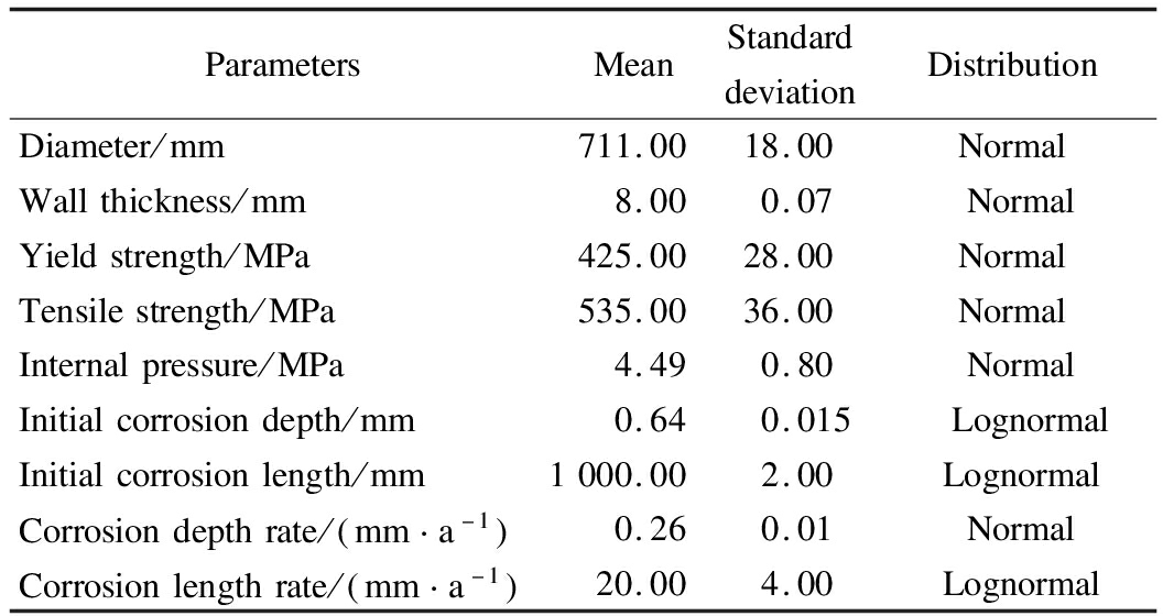
ParametersMeanStandarddeviationDistributionDiameter/mm711.0018.00NormalWallthickness/mm8.000.07NormalYieldstrength/MPa425.0028.00NormalTensilestrength/MPa535.0036.00NormalInternalpressure/MPa4.490.80NormalInitialcorrosiondepth/mm0.640.015LognormalInitialcorrosionlength/mm1000.002.00LognormalCorrosiondepthrate/ mm a-1 0.260.01NormalCorrosionlengthrate/ mm a-1 20.004.00Lognormal
3.1 Burst pressure simulation and experimental verification
For the pipeline, its stress and deformation distribution can be obtained with FEM simulation, as shown in Fig.1.To verify the accuracy of the simulation results, a hydraulic burst test is conducted to obtain the pipeline burst pressure, and the corresponding test platform is shown in Fig.2.Moreover, the pipeline’s burst pressure is also calculated with international criteria, including the B31Gmod, DNV RP-F101, SHELL92, and PCORRC, as shown in Fig.3.According to the four international criteria, the calculated burst pressure shows a downward trend with the increase ofd/t, i.e., the ratio of the defect depth(d)to the wall thickness(t).The observed trend is consistent with the actual situation.
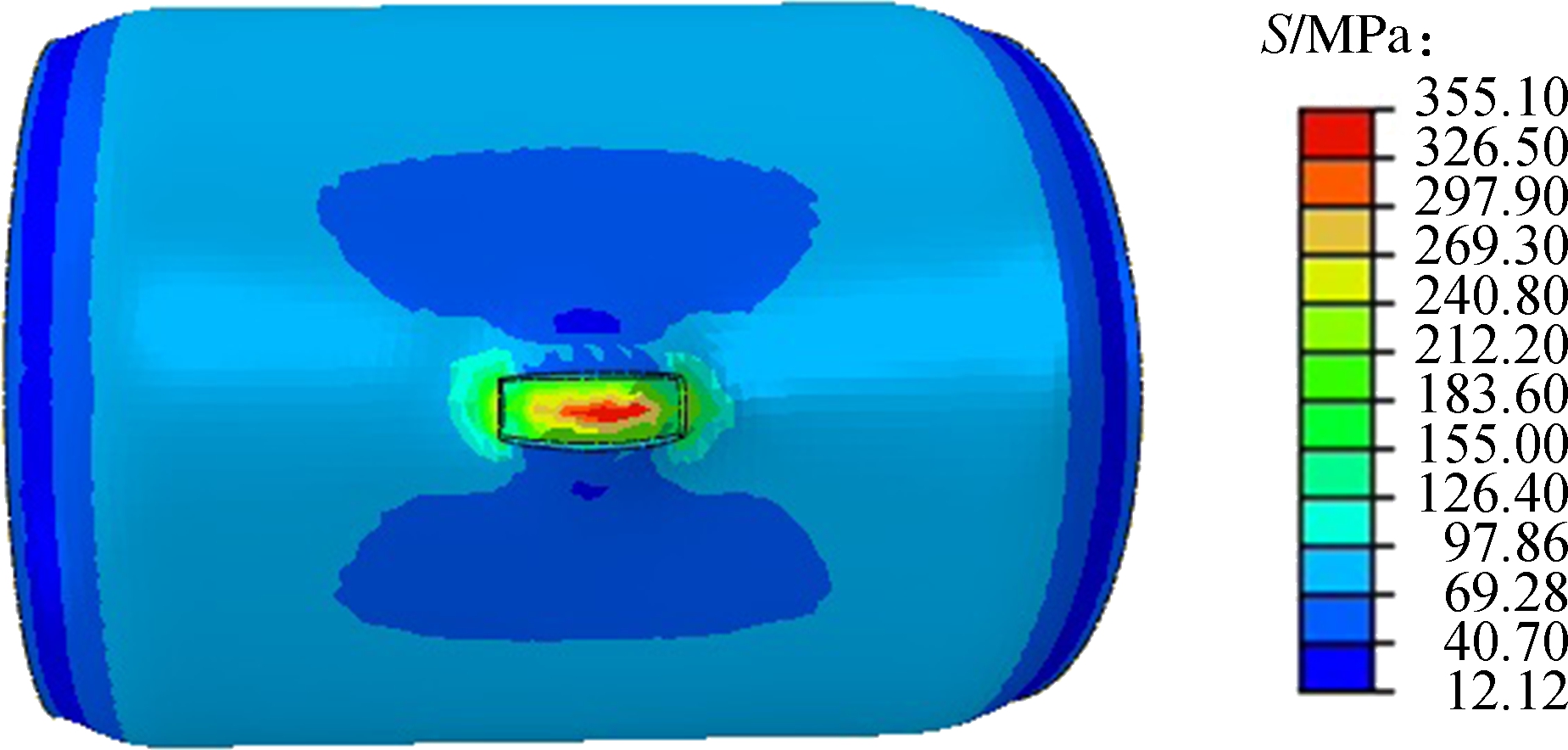
Fig.1 Cloud diagrams of the pipeline’s stress
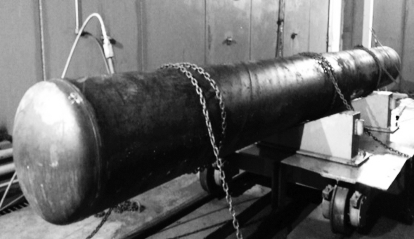
Fig.2 Hydraulic burst test for the pipeline
From Fig.3, the results obtained with FEM are very close to the results of field test, with a maximum error of 10.7%.According to the degree of closeness between the calculated results of the criteria as well as the result of the field test, the rank order from the best to the worst is PCORRC, DNV RP-F101, B31Gmod, SHELL92.Moreover, even though the results of the PCORRC are closer to the test results, the maximum error is still as high as 18.4%.Thus, compared with the results of the criteria, more accurate burst pressure can be obtained with FEM.
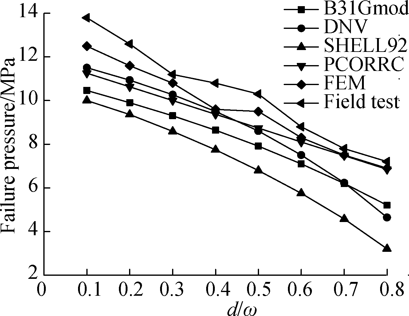
Fig.3 Comparison of the pipeline’s failure pressures
3.2 Determination of the corrosion growth
On the basis of Eqs.(2)and(4), the linear corrosion growth model is obtained, i.e., d(t)=0.8ω-(d0+0.13t).The parameters in Eqs.(7)and(8)are set as follows: k0=0.608; k1=-0.000 18; k2=-0.065 4; k3=-0.000 26; k4=0.000 874; k5=-0.000 639; k6=-0.000 122; α0=0.896; α1=0.519; α2=0.004 65; α3=-0.099; and α4=0.431[25].Based on Eqs.(6)to(8)and Tab.2, the expression of power-law function for the corrosion growth model is obtained, i.e., d(t)=0.094(t-3)0.88.Fig.4 shows the failure probability curves that are obtained with the linear growth model and power-law function growth model.
Tab.2 Parameters of the soil environmental variables of pipelines
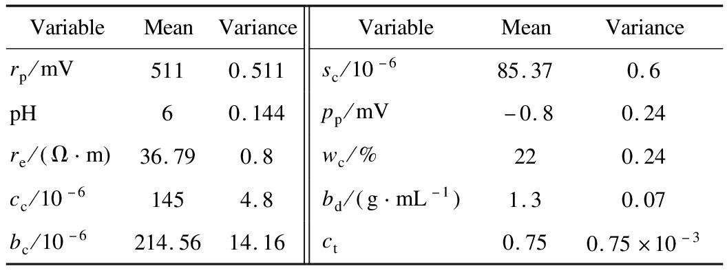
VariableMeanVarianceVariableMeanVariancerp/mV5110.511sc/10-685.370.6pH60.144pp/mV-0.80.24re/ Ω m 36.790.8wc/%220.24cc/10-61454.8bd/ g mL-1 1.30.07bc/10-6214.5614.16ct0.750.75×10-3
As shown in Fig.4, the predicted results of the two models have similar variation tendency.With the increase of the running time, the probability that the pipeline may fail tends to increase.However, the predicted failure probability with the linear model is smaller than the result of the power-law function model.Thus, the power-law function model is more suitable, and more accurate results can be obtained with considering the environmental factors.
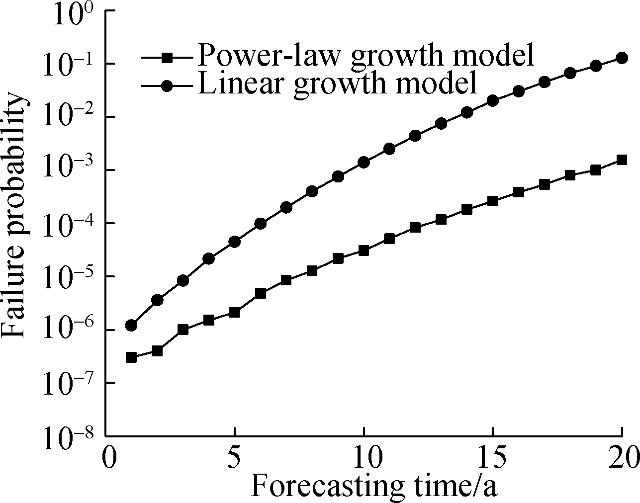
Fig.4 Failure curves of the pipeline with corrosion
3.3 Comparison of corrosion failure probabilities
Fig.5 shows the failure probability calculated with different models.Obviously, there is a difference among the prediction results.The largest failure probability is obtained with the SHELL92 model, which will result in a smaller estimation of the burst pressure.
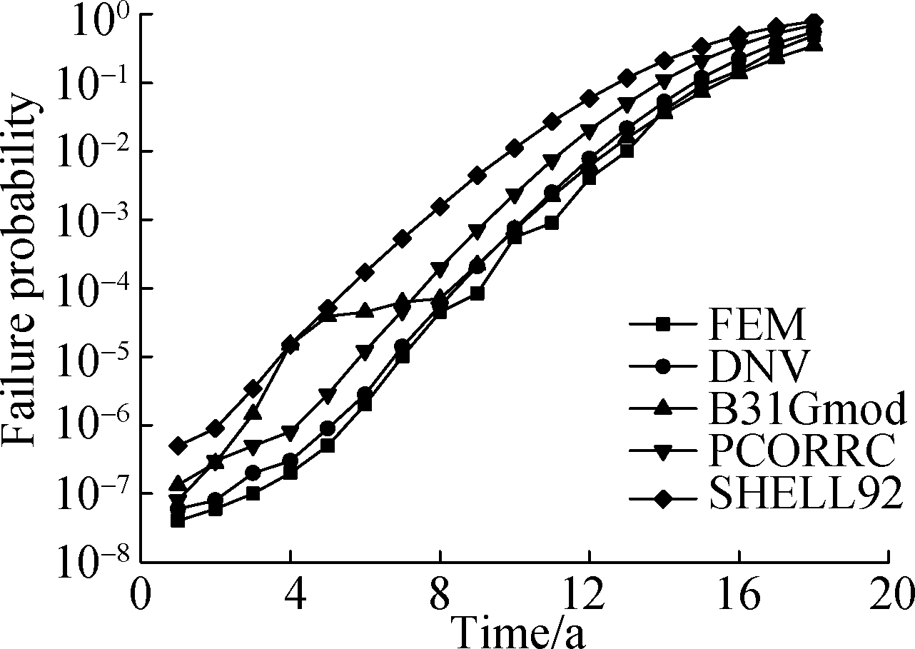
Fig.5 Failure probability curves under different calculation models
Fig.3 shows that the predicted result with FEM is closest to the test result, followed by DNV RP-F101, PCORRC, B31Gmod, and SHELL92.Moreover, in terms of failure rate prediction, the prediction result of FEM is also the smallest, followed by DNV RP-F101, PCORRC, B31Gmod, and SHELL92.
The pipeline is considered to be failed, when either of the two types of failure occurs.Thus, we can obtain the pipeline’s RUL according to the maximum acceptable failure probability.As shown in Fig.4, a failure rate of 10-4 corresponds to a residual life of about 13 years and 7 years based on the power-law function growth model and linear growth model, respectively.The predicted RUL obtained with the linear growth model is shorter than that of the power-law function growth model.The result is observed to be conservative.
3.4 Sensitivity analysis of the parameters
Considering that a variety of factors can affect the pipeline’s failure probability, it is crucial to find the key parameters(e.g., diameter and wall thickness of the pipeline, operation pressure, and corrosion rate in different directions)to predict the pipeline’s failure probability or RUL more accurately, or to prolong the service time and properly draw up a maintenance policy.Here, the coefficient of variation is used to characterize the sensitivity of the parameters, as follows:
(11)
Fig.6 shows the pipeline’s failure rate change with the initial corrosion depth.When the variation coefficient of the initial corrosion depth(i.e., cov(d0))changes from 0.01 to 0.3, the failure rate curve remains unchanged.This indicates that the initial corrosion depth of defects has little influence on the failure rate.Moreover, the failure rate change with the axial corrosion rate has a similar tendency.
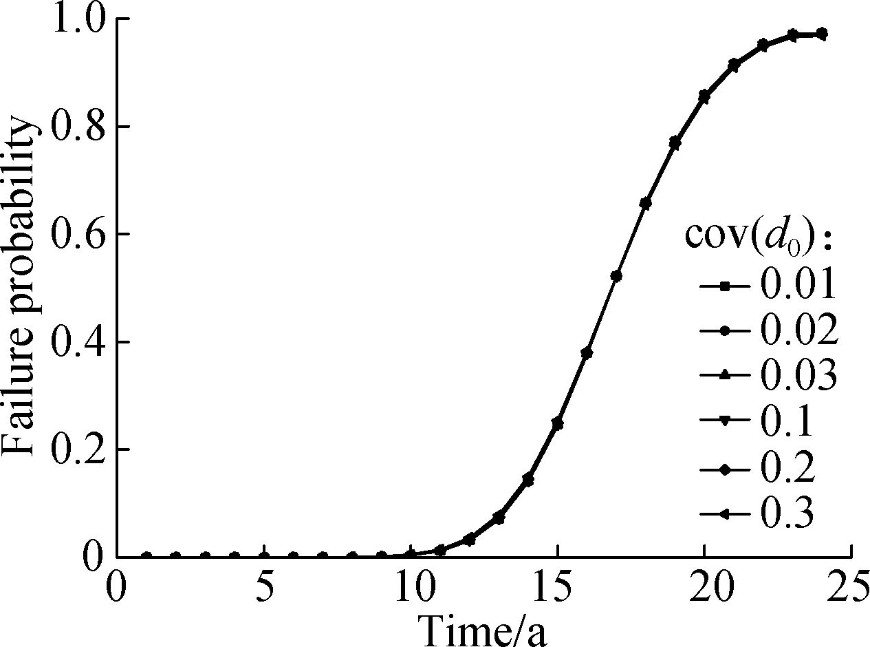
Fig.6 Failure probability curve under different cov(d0)
Figs.7 and 8 show the pipeline’s failure rate changes with the tensile strength and diameter, respectively.It can be seen that these two parameters have certain influences on the failure rate.
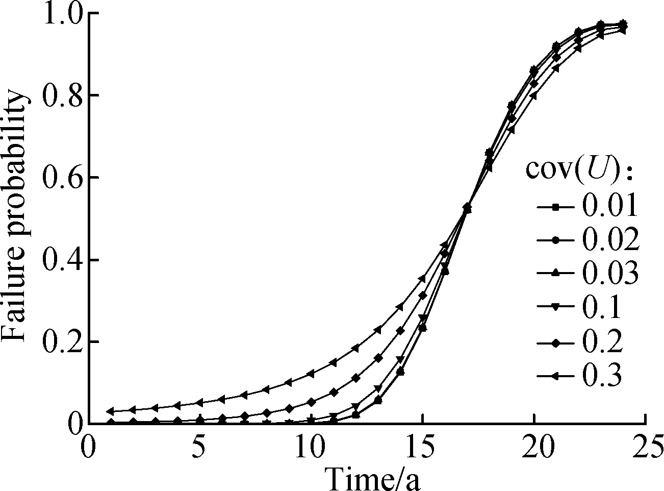
Fig.7 Failure probability curve under different cov(U)
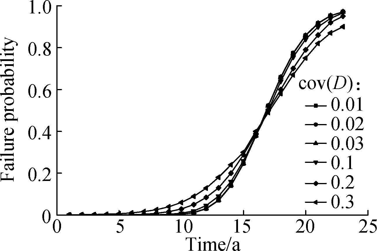
Fig.8 Failure probability curve under different cov(D)
Moreover, sensitivity analysis for other parameters, including the radial corrosion rate of defects, the length and wall thickness of the pipeline, and the operating pressure, are also implemented.The results for the above parameters are not discussed detailedly here.It is found that the radial corrosion rate, wall thickness, and operating pressure are closely related to the limit state equation.Moreover, the defect’s length has some effect on the pipeline’s failure rate.However, the effect is not so obvious.
4 Conclusions
1)This study integrates FEM and MCS to predict the pipeline’s RUL, and a case study is conducted to analyze the law of corrosion defect’s size change over time.Moreover, the accuracy of the proposed method is verified with the results of hydraulic burst test and major international criteria.
2)Compared with the results obtained with linear growth model, more accurate results can be obtained by using the power-law function model.
3)Sensitivity analysis is implemented for the parameters.The results show that the radial corrosion rate, wall thickness, and operating pressure have obvious impact on the failure of the pipeline.Furthermore, as these parameters may correlate with each other, it can be taken into account in future research.
[1] Wang Y H, Zhang P, Qin G J.Reliability assessment of pitting corrosion of pipeline under spatiotemporal earthquake including spatial-dependent corrosion growth[J].Process Safety and Environmental Protection, 2021, 148:166-178.DOI:10.1016/j.psep.2020.10.005.
[2] Mahmoodian M, Li C Q.Failure assessment and safe life prediction of corroded oil and gas pipelines[J].Journal of Petroleum Science and Engineering, 2017, 151:434-438.DOI:10.1016/j.petrol.2016.12.029.
[3] Wang W H,Shen K L, Wang B B, et al.Failure probability analysis of the urban buried gas pipelines using Bayesian networks[J].Process Safety and Environmental Protection, 2017, 111:678-686.DOI:10.1016/j.psep.2017.08.040.
[4] Mosallam A, Medjaher K, Zerhouni N.Data-driven prognostic method based on Bayesian approaches for direct remaining useful life prediction[J].Journal of Intelligent Manufacturing, 2016, 27(5):1037-1048.DOI:10.1007/s10845-014-0933-4.
[5] Gong C Q, Zhou W X.First-order reliability method-based system reliability analyses of corroding pipelines considering multiple defects and failure modes[J].Structure and Infrastructure Engineering, 2017, 13(11):1451-1461.DOI:10.1080/15732479.2017.1285330.
[6] Nahal M, Chateauneuf A, Sahraoui Y.Reliability analysis of irregular zones in pipelines under both effects of corrosion and residual stress[J].Engineering Failure Analysis, 2019, 98:177-188.DOI:10.1016/j.engfailanal.2019.01.081.
[7] Bouledroua O, Zelmati D, Hassani M.Inspections, statistical and reliability assessment study of corroded pipeline[J].Engineering Failure Analysis, 2019, 100:1-10.DOI:10.1016/j.engfailanal.2019.02.012.
[8] Hasan S, Khan F, Kenny S.Probability assessment of burst limit state due to internal corrosion[J].International Journal of Pressure Vessels and Piping, 2012, 89:48-58.DOI:10.1016/j.ijpvp.2011.09.005.
[9] Leira B J, Næss A, Brandrud Næss O E.Reliability analysis of corroding pipelines by enhanced Monte Carlo simulation[J].International Journal of Pressure Vessels and Piping, 2016, 144:11-17.DOI:10.1016/j.ijpvp.2016.04.003.
[10] Mohamed E A B S, Keshtegar B, Correia J A F O, et al.Reliability analysis based on hybrid algorithm of M5 model tree and Monte Carlo simulation for corroded pipelines:Case of study X60 Steel grade pipes[J].Engineering Failure Analysis, 2019, 97:793-803.DOI:10.1016/j.engfailanal.2019.01.061.
[11] Tee K F, Khan L R.Reliability analysis of underground pipelines with correlations between failure modes and random variables[J].Proceedings of the Institution of Mechanical Engineers, Part O:Journal of Risk and Reliability, 2014, 228(4):362-370.DOI:10.1177/1748006x13520145.
[12] Mondal B C, Dhar A S.Finite-element evaluation of burst pressure models for corroded pipelines[J].Journal of Pressure Vessel Technology, 2017, 139(2):021702.DOI:10.1115/1.4034408.
[13] Zelmati D, Ghelloudj O, Amirat A.Reliability estimation of pressurized API 5L X70 pipeline steel under longitudinal elliptical corrosion defect[J].The International Journal of Advanced Manufacturing Technology, 2017, 90(9/10/11/12):2777-2783.DOI:10.1007/s00170-016-9580-6.
[14] Shuai Y, Shuai J, Xu K.Probabilistic analysis of corroded pipelines based on a new failure pressure model[J].Engineering Failure Analysis, 2017, 81:216-233.DOI:10.1016/j.engfailanal.2017.06.050.
[15] Nahal M, Khelif R, Bourenane R, et al.Pipelines reliability analysis under corrosion effect and residual stress[J].Arabian Journal for Science and Engineering, 2015, 40(11):3273-3283.DOI:10.1007/s13369-015-1723-9.
[16] Tee K F, Khan L R, Li H S.Application of subset simulation in reliability estimation of underground pipelines[J].Reliability Engineering & System Safety, 2014, 130:125-131.DOI:10.1016/j.ress.2014.05.006.
[17] Al-Amin M, Zhou W X.Evaluating the system reliability of corroding pipelines based on inspection data[J].Structure and Infrastructure Engineering, 2014, 10(9):1161-1175.DOI:10.1080/15732479.2013.793725.
[18] Ossai C I, Boswell B, Davies I.Markov chain modelling for time evolution of internal pitting corrosion distribution of oil and gas pipelines[J].Engineering Failure Analysis, 2016, 60:209-228.DOI:10.1016/j.engfailanal.2015.11.052.
[19] Pesinis K, Tee K F.Statistical model and structural reliability analysis for onshore gas transmission pipelines[J].Engineering Failure Analysis, 2017, 82:1-15.DOI:10.1016/j.engfailanal.2017.08.008.
[20] Gong C, Zhou W.Importance sampling-based system reliability analysis of corroding pipelines considering multiple failure modes[J].Reliability Engineering & System Safety, 2018, 169:199-208.DOI:10.1016/j.ress.2017.08.023.
[21] Wen K, He L, Liu J, et al.An optimization of artificial neural network modeling methodology for the reliability assessment of corroding natural gas pipelines[J].Journal of Loss Prevention in the Process Industries, 2019, 60:1-8.DOI:10.1016/j.jlp.2019.03.010.
[22] Palencia O G, Teixeira A P,Guedes Soares C.Safety of pipelines subjected to deterioration processes modeled through dynamic Bayesian networks[J].Journal of Offshore Mechanics and Arctic Engineering, 2019, 141(1):011602.DOI:10.1115/1.4040573.
[23] Wang Y F, Su C, Xie M J.Remaining useful life prediction of corroded oil pipelines based on binary inverse Gaussian process[J].Journal of Southeast University(Natural Science Edition), 2020, 50(6):1038-1044.DOI:10.3969/j.issn.1001-0505.2020.06.007.(in Chinese)
[24] Li J, Liang B Q, Li C, et al.Calculation methods for the gas pipeline failure rate[J].Journal of Petroleum Science and Engineering, 2019, 174:229-234.DOI:10.1016/j.petrol.2018.11.020.
[25] Zhang P, Su L B, Qin G J, et al.Failure probability of corroded pipeline considering the correlation of random variables[J].Engineering Failure Analysis, 2019, 99:34-45.DOI:10.1016/j.engfailanal.2019.02.002.
[26] Aljaroudi A, Thodi P, Akinturk A, et al.Probabilistic methods for predicting the remaining life of offshore pipelines[J].Journal of Pressure Vessel Technology, 2017, 139(4):041701.DOI:10.1115/1.4036217.
[27] Liu A H, Chen K, Huang X F, et al.Corrosion failure probability analysis of buried gas pipelines based on subset simulation[J].Journal of Loss Prevention in the Process Industries, 2019, 57:25-33.DOI:10.1016/j.jlp.2018.11.008.
[28] Velázquez J C,Caleyo F, Valor A, et al.Predictive model for pitting corrosion in buried oil and gas pipelines[J].Corrosion, 2009, 65(5):332-342.DOI:10.5006/1.3319138.
[29] Siraj T, Zhou W X.Evaluation of statistics of metal-loss corrosion defect profile to facilitate reliability analysis of corroded pipelines[J].International Journal of Pressure Vessels and Piping, 2018, 166:107-115.DOI:10.1016/j.ijpvp.2018.08.007.
[30] Abdelghani M, Tewfik G, Djahida D, et al.Prediction of the rupture pressure of transmission pipelines with corrosion defects[J].Journal of Pressure Vessel Technology, 2018, 140(4):041701.DOI:10.1115/1.4039698.
[31] Su C, Wang S J,Xu Y Q.Dynamic reliability of hydraulic system based on Monte Carlo simulation[J].Journal of Southeast University(Natural Science Edition), 2006, 36(3):370-373.DOI:10.3321/j.issn:1001-0505.2006.03.007.(in Chinese)