Existing studies show that the air suspension system using air springs improves cars’ ride quality better than the traditional suspension system using steel springs[1-2]. Semi-active air suspensions (SASs) use the fuzzy control (FC) and Hinf control methods[3-4] to ameliorate cars’ ride quality. Investigations indicated that SASs controlled by the FC significantly ameliorated cars’ ride quality when compared to the passive suspension system. Moreover, the investigations showed that the efficiency of the FC is greatly affected by its control rules, which is also considered its disadvantage. To enhance the efficiency of the FC, its control rules were then optimized based on the genetic algorithm (GA)[3, 5-6]. The study results indicated that the efficiency of an FC used with optimized control rules is better than that of an FC without optimized control rules. However, the harmonic excitation or random excitation of rigid roads was mainly applied to evaluate the efficiency of the FC and cars’ ride comfort in the above studies.
The SAS efficiency controlled by an FC with its optimized control rules under random surfaces of the ISO levels A, B, C, D, and E of a rigid road[7] was investigated[3, 8]. The studies indicated that an FC with optimized control rules was only effective under each excitation of the ISO level A, B, C, D, or E of a rigid road surface. The control efficiency of an FC significantly decreased when the vehicle was moving along random surfaces of a rigid road changed in a large range. In addition, with the deformable surfaces of a soft road, its deformation was also changed in a large range when the vehicle was moving on the soft road[9-10]. However, the influence of soft roads on cars’ ride quality and SAS efficiency is less studied. Moreover, some studies on the elastic tire-soft road interaction indicated that vibration sources under an elastic tire are not only generated by a random surface but also by the deformable terrain of a soft road. Therefore, cars’ ride quality is strongly influenced by the vibration sources of soft roads[9, 11]. Hence, the FC efficiency and its control rule optimization can also be affected by soft road surfaces. However, this issue has not yet been concerned in existing studies.
A machine learning (ML) method is being investigated and used in adaptive controls. Based on the desired input data and output data of a machine system and an FC, a self-learning algorithm program[12-13] could be developed to control cars’ suspension systems under various simulation conditions. This topic is currently of particular interest to scholars. Thus, based on cars’ dynamic model and the control rules of an FC optimized by a GA on soft and rigid roads, an ML program was investigated and developed for optimizing SAS efficiency and cars’ ride quality. The root-mean-square (RMS) acceleration responses of the driver’s seat (awz1) and car’s pitch angle (awφ2) were chosen as the objective functions. The goal of the study is to enhance cars’ ride quality under soft and rigid roads.
1 Mathematical Approaches
1.1 Car dynamic model
A car dynamic model with its suspension system used by an SAS was established to control it via ML, as shown in Fig. 1. In the figure, zi and mi are the vertical displacements and masses of the driver’s seat, car body, and axles, respectively; φ2 is the angular displacement of the car body; c1, ct1,2, and kt1,2 are the damping and stiffness values of the seat suspension and wheels; q1,2 are the excitations at the front and rear wheels; lj is the distances of the car; and v0 is the car’s moving velocity (i=1, 2, 3, 4; j=1, 2, 3).

Fig.1 Lumped model of the car
To simplify the computation process of the car’s motion equations, some assumptions are given as follows: 1) The car body is absolutely stiff, and its angular deformation is very small and hence ignored. 2) The displacements of the seat, car body, and axles around their equilibrium position are very small. 3) The vibration excitation is mainly in the vertical direction, and the longitudinal and horizontal excitations are very small and hence ignored. Based on the car’s dynamic model in Fig. 1 and Newton’s second law of motion, the general dynamic differential equation for the car is given by
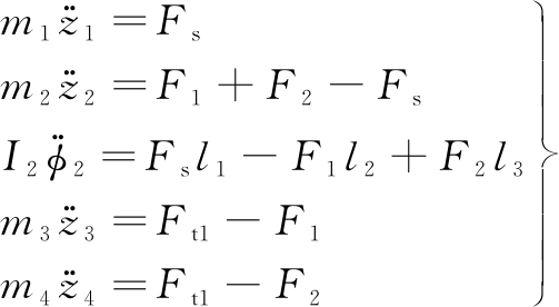
(1)
where Fs is the vertical force of the driver’s seat suspension system, written as
(2)
F1 and F2 are the vertical forces of the front and rear SASs, respectively. Ft1 and Ft2 are the vertical forces of the front and rear wheels, respectively.
1.2 Dynamic model of the SAS
To evaluate the ML efficiency in controlling the car’s SAS, the SAS used by an airbag spring and an active damper controlled by the FC were applied. The SAS simple structure includes a bag and reservoir connected by a surge pipe, as described in Fig. 2(a), where Vb, pb, and Ae are the volume, pressure, and effective area of the airbag, respectively; As, ms, and ls are the cross-sectional area, air mass, and length of the pipe, respectively; Vr and pr are the volume and pressure of the reservoir, respectively; z is the deformation of the airbag; and υs is the air displacement of the air in the pipe.
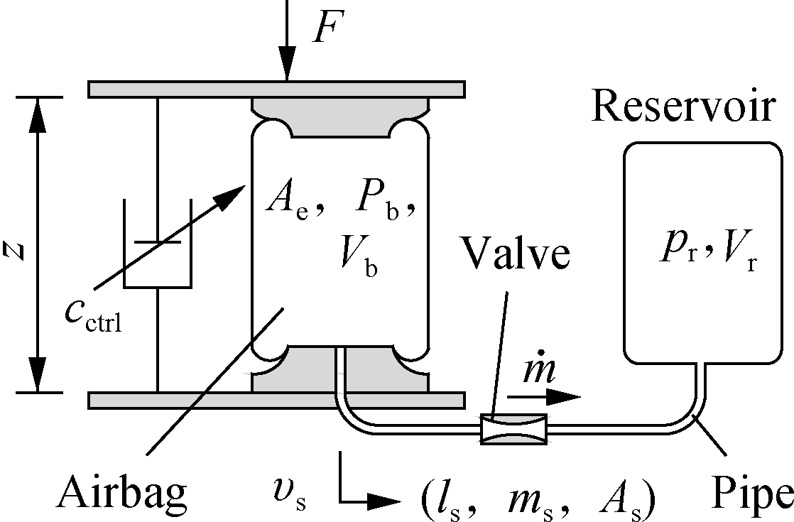
(a)
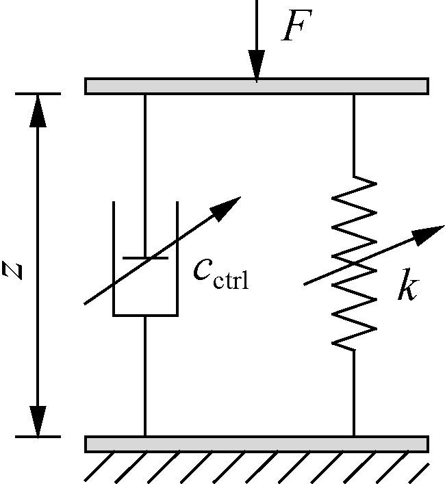
(b)
Fig.2 SAS model. (a) SAS structure; (b) Dynamic model
Some assumptions of the SAS model are given as follows: 1) the friction of the airbag’s material is very small; 2) the inertia force of the air mass in the SAS is also very small and neglected; and 3) the vibration excitation of the SAS model is mainly in the vertical direction.
The force balance between F and the restoring force of the airbag in Fig. 2(a) is expressed as
F=Ae(pb-pa)
(3)
where pa is the atmospheric pressure.
Based on the correlation among the reservoir, pipe, and airbag, pb is computed by the air mass flow rate into the airbag as follows:
(4)
The relationship of ρb and pb was calculated based on the isentropic process in the airbag as follows[2]:
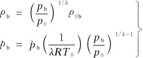
(5)
where ρ0b is the air density at the initial state and is determined by ρ0b=p0/(RT0) and λ is the polytropic constant, λ=1.4[3, 8].
By combining Eqs. (4) and (5), ![]() is calculated by
is calculated by

(6)
The air mass flow rate into the reservoir is written as
(7)
Based on the relationship between ρr and pr in the reservoir, ![]() is determined by
is determined by

(8)
By combining Eqs. (7) and (8), ![]() is calculated by
is calculated by
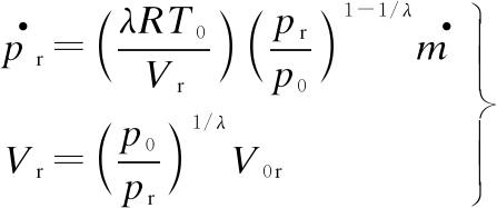
(9)
The mass flow rate in the pipe is also expressed as
(10)
In addition, the mass flow rate of the air in the pipe was affected by As, pr, and pb of the air suspension system[3]. Thus, the moving air mass in the pipe is written as[3]
(11)
By combining Eqs. (10) and (11), the mass flow rate in the pipe is expressed as
(12)
By combining Eqs. (6), (9), and (12), pb and F in Eq. (3) can be determined.
Based on the derivative of F/z, the SAS nonlinear dynamic stiffness can be calculated as
(13)
Based on the ideal gas state equation of the ![]() we have
we have
(14)
By substituting Eq. (14) into Eq.(13), k is then rewritten as
(15)
The SAS dynamic model is described in Fig. 2(b).
From the car and SAS models given in Figs. 1 and 2(b), the vertical forces of the front/rear SAS are expressed as
k1(zi+1-z2+φ2li+1) i=1,2
(16)
where cctrli is the damping values of the front/rear SAS.
1.3 Models of the wheel-road surface contact
1.3.1 Contact model of the wheel-soft road surface
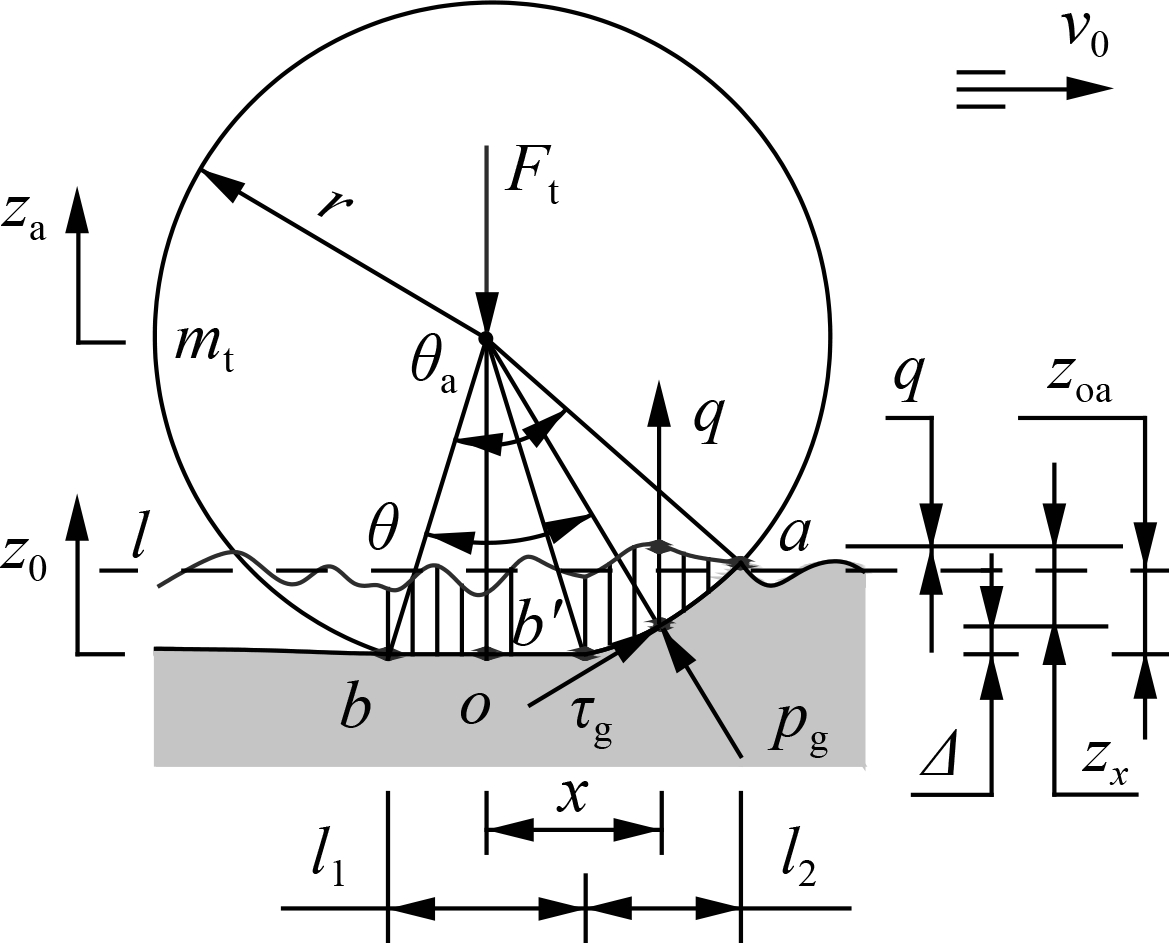
When the car is traveling on the soft road surface, the elastic wheel interacts with the soft road. A dynamic model of the wheel-soft road interaction with the surface roughness of the soft road q is built in Fig. 3(a). Under the effect of the dynamic and static loads of the wheel on the soft road surface, the road surface is sunk by zoa. Two deformable regions of the soft road surface-wheel (bob′ region) and soft road surface (b′a region) appeared, as shown in Fig. 3(a). zx, z0, and za are the sinkage of the soft road, static deformation of the soft road, and axle displacement, respectively, and r, Ft, and mt are the radius, dynamic force, and mass of the wheel, respectively.
(a)
(b)
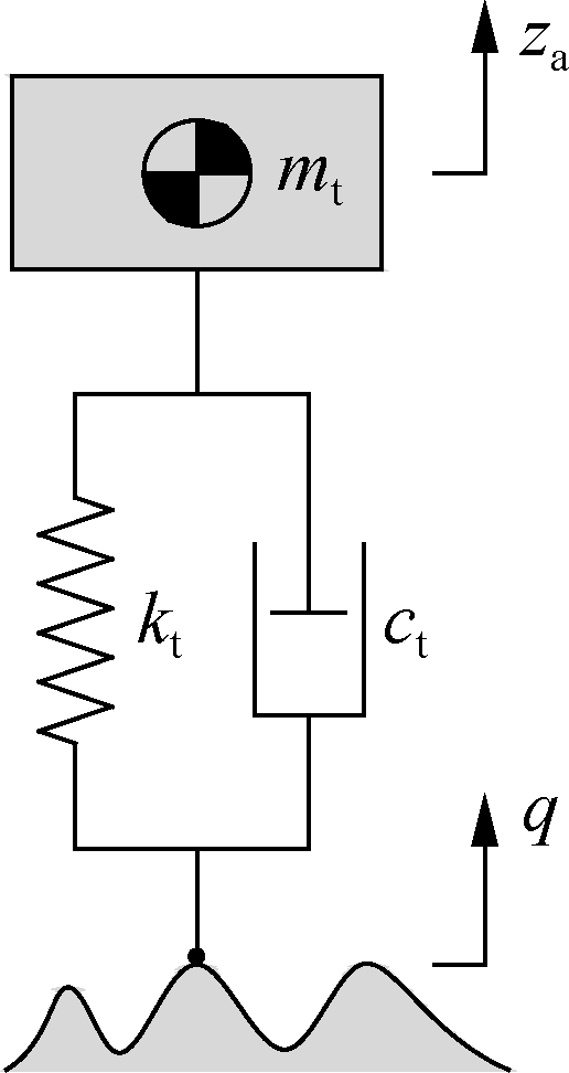
Fig.3 Contact model of the elastic wheel-road surface. (a) Soft road; (b) Rigid road
Assuming that the contact lengths of bob′ and b′a in the horizontal direction are l1 and l2, respectively, the pressure pg and shear stress τg of the soft road generated in the contact lengths l1 and l2 are described by the reaction force of the soft road on the elastic wheel as follows[9]:
τg=(c+pgtanφ)(1-e-j/K)
(17)
where ![]() kφ and kc are the stiffness values of the internal friction and sinkage, respectively; b and n are the dimension and sinkage exponent of the contact patch, respectively; c and φ are the soil cohesion coefficient and internal friction angle, respectively; and K is the shear deformation modulus.
kφ and kc are the stiffness values of the internal friction and sinkage, respectively; b and n are the dimension and sinkage exponent of the contact patch, respectively; c and φ are the soil cohesion coefficient and internal friction angle, respectively; and K is the shear deformation modulus.
It is assumed that l is the average roughness line of the soft road surface, so zx can be determined by
zx=zoa+q+zoa-Δ=za-z0+q+Ψ-r
(18)
The force responses at the front and rear axles of the elastic wheel are determined by
(19)
where g is the gravitational acceleration and i=1, 2.
To determine q in Eq. (18), the power spectrum density G(w0) of the soft road surface roughness was calculated as[3, 10]
(20)
where w0 = 0.1 m is the reference frequency.
Based on the white noise signal W and G(f), q is then determined by[14]
(21)
Mitschke[10] presented the spectral densities of soft road classifications, including good, medium, and poor soil surfaces, as provided in Tab. 1. Thus, q is generated using a parameter in these spectral densities.
Tab.1 Parameters of the soft road surface

Level surfacesδG(w0)/ (10-6 m3·cycle-1)Good2.55199.8Medium2.55973.9Poor2.143 782.5
1.3.2 Contact model of the wheel-rigid road surface
When a car is traveling on a rigid road surface, the surface greatly affects the car’s ride quality. Here, the point-contact model of the rigid road-wheel interaction was used to calculate the force response of the wheel[5, 14-15]. To calculate the force response of the wheel, the point-contact model of the rigid road surface-wheel interaction is also established in Fig. 3(b).
The vertical forces of the front and rear wheels (Fti) are written as
(22)
q of the rigid road surface is computed in Eq. (21) with G(w0) determined according to ISO-8068[7].
1.4 Evaluating index
To estimate the driver’s ride quality and the efficiency of isolation systems, the index of the RMS accelerations of the seat calculated according to ISO 2631-1[16] was used[6, 8, 14]. Based on the car’s dynamic model and ISO 2631-1, the RMS accelerations of the driver’s seat and car’s pitch angle are written as
(23)
where χ={z1, φ2}; aχ(t) is the acceleration in κ; and T is the simulation time.
To assess SAS efficiency controlled by the ML model on enhancing the car’s ride quality under various surfaces of soft and rigid roads, the decrease in awz1 and awφ2 was chosen as the evaluation index.
2 SAS Control Algorithm
The FC efficiency greatly depends on its control rules. The control rules of the FC are also optimized by the GA to enhance its efficiency[6]. However, the optimized control rules also strongly depend on the conditions of the road surface and car speed. The FC efficiency could be reduced when the high roughness of the road surface is changed in a large range. To overcome this shortcoming, based on the various surfaces of a soft road, including good, medium, and poor soil surfaces[10], and various surfaces of a rigid road, including level A, level B, and level C, according to the ISO 8068[7], each control rule of a road surface was optimized. Then, a data map of the FC control rules optimized under all the soft and rigid roads was applied for the ML model to control cctrl.
2.1 Optimizing the FC control rules
The structure of FCs is defined by the fuzzification interface (FI), fuzzy inference system (FIS), and defuzzification interface (DI). First, input values in the FI were transformed into linguistic variables (LV). Then, the FIS was used to compute the LV using deductive rules. Finally, the LV was transformed back to the output values via the DI for controlling the objectives[3, 6]. To control the front and rear SASs, two damping values of cctrl1 and cctrl2 should be separately controlled. Thus, two controllers should be designed. However, the design process of the FC for the front and rear SASs is the same. Thus, a specific FC was designed and applied to control the front and rear SASs. To design the FC, the displacement z and velocity ![]() of the SASs are two input values, while cctrl is an output value. The LV and values of z,
of the SASs are two input values, while cctrl is an output value. The LV and values of z, ![]() and cctrl provided in Tab. 2 were used to build the membership function of the FC input/output variables.
and cctrl provided in Tab. 2 were used to build the membership function of the FC input/output variables.
Tab.2 LV input/output and value of the FC
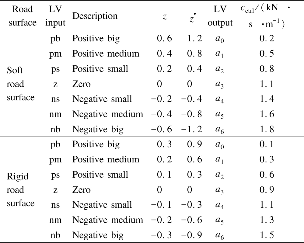
Road surfaceLV inputDescriptionzz·LV outputcctrl/(kN·s·m-1)Soft road surfacepbPositive big0.61.2a00.2pmPositive medium0.40.8a10.5psPositive small0.20.4a20.8zZero00a31.1nsNegative small-0.2-0.4a41.4nmNegative medium-0.4-0.8a51.6nbNegative big-0.6-1.2a61.8Rigid road surfacepbPositive big0.30.9a00.1pmPositive medium0.20.6a10.3psPositive small0.10.3a20.6zZero00a30.9nsNegative small-0.1-0.3a41.1nmNegative medium-0.2-0.6a51.3nbNegative big-0.3-0.9a61.5
Based on the LV and values of z, ![]() and cctrl of the soft and rigid roads defined in Tab. 2, the “if-then” control rule in the FIS is described as follows:
and cctrl of the soft and rigid roads defined in Tab. 2, the “if-then” control rule in the FIS is described as follows:
1) If z=pb and ![]() then cctrl=a0.
then cctrl=a0.
2) If z=pb and ![]() then cctrl=a1.
then cctrl=a1.
…
49) If z=nb and ![]() then cctrl=a6.
then cctrl=a6.
To enhance the FC efficiency, the GA was then applied to optimize the “if-then” rule as follows.
The input variables ![]() pm, ps, z, ns, nm, nb of the LV were encoded by [ui]1×7; the output variables cctrl=a0, a1, …, a6 of the LV were also encoded by [vj]1×7; and the GA population initialization was 150. The individuals of x=[ui vj]T created in the initial population were random, and each gene in ui and vi was randomly selected from pb to nb and a0 to a6. The fitness value of the GA given by the minimum value of Jmin=min{awz1, awφ2} was then applied to optimize the FC control rules. Through the GA optimal process, the individuals of x that create low Jmin will provide good control rules. Then, these individuals were updated and optimized until the evolutionary generation of 1 500 ended or satisfied the stop condition of |Jmin(i+1)-Jmin(i)|≤0.001 of the GA.
pm, ps, z, ns, nm, nb of the LV were encoded by [ui]1×7; the output variables cctrl=a0, a1, …, a6 of the LV were also encoded by [vj]1×7; and the GA population initialization was 150. The individuals of x=[ui vj]T created in the initial population were random, and each gene in ui and vi was randomly selected from pb to nb and a0 to a6. The fitness value of the GA given by the minimum value of Jmin=min{awz1, awφ2} was then applied to optimize the FC control rules. Through the GA optimal process, the individuals of x that create low Jmin will provide good control rules. Then, these individuals were updated and optimized until the evolutionary generation of 1 500 ended or satisfied the stop condition of |Jmin(i+1)-Jmin(i)|≤0.001 of the GA.
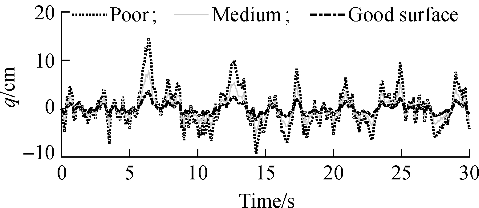
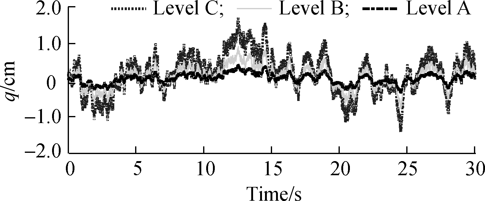
To optimize the FC control rules and establish a data map for the ML model under soft and rigid roads, the values of δ and G(w0) of the soft road surfaces in Tab. 1, f<10 Hz, and v0=54 km/h were applied to build the various surfaces of the soft road. Moreover, the rigid road surfaces of levels A (good), B (medium), and C (poor) of G(w0), δ=2, f<10 Hz, and v0=54 km according to ISO-8068[7] were applied to build the various surfaces of the rigid road. The simulation results of the soft and rigid roads with various surfaces are plotted in Figs. 4(a) and (b).
(a)
(b)
Fig.4 Random road surfaces. (a) Soft road; (b) Rigid road
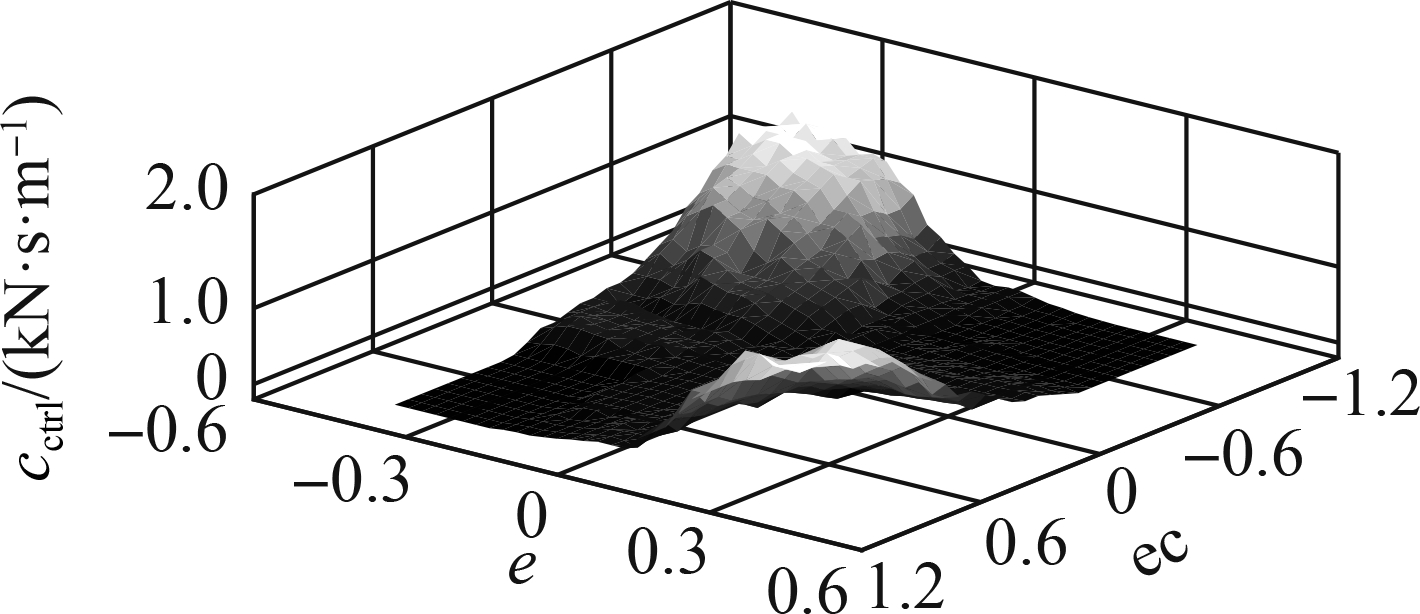
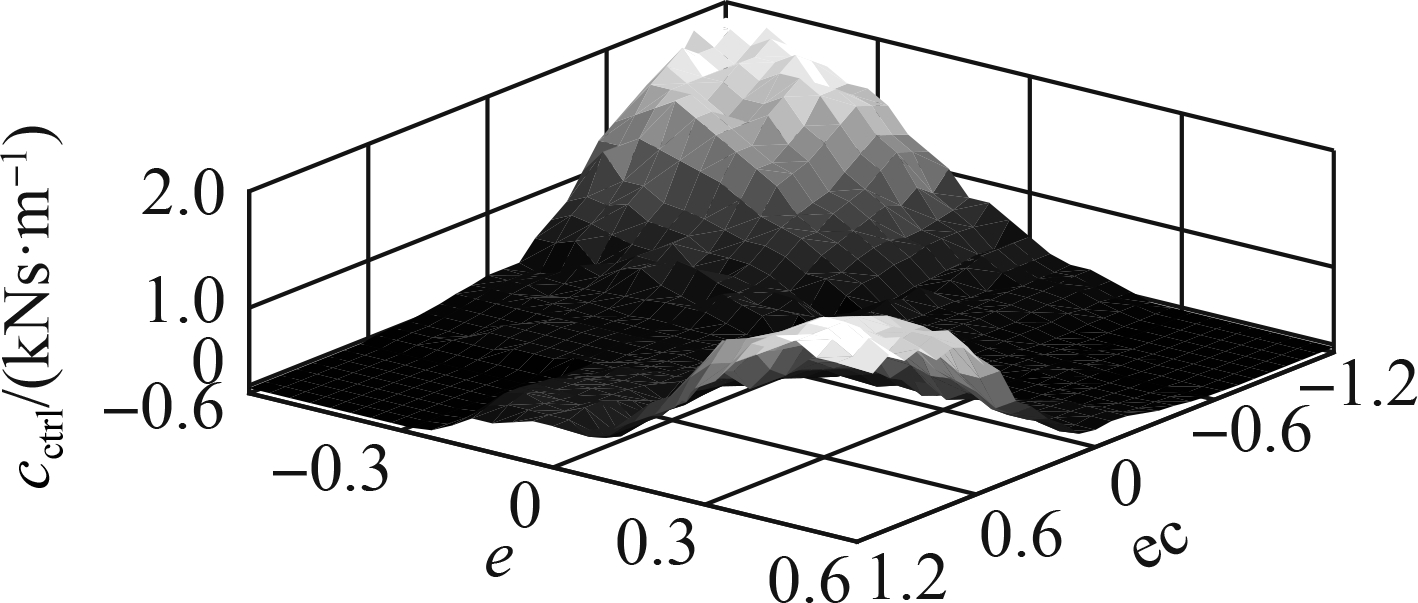
Based on the different vibration excitations of q in Fig. 4, initial control rules of the FC in Tab. 2, and car’s dynamic parameters in Tab. 3, an algorithm program was then built to optimize the FC control rules, as plotted in Fig. 5 with “FC.” From the optimized control rules of the FC, three different types of data map, namely, 1) using the good, medium, and poor soil surfaces of the soft road; 2) using the surface of ISO levels A, B, and C of the rigid road; and 3) using the soft and rigid road surfaces, are plotted in Fig. 6.
Tab.3 Dynamic parameters of the car and SAS

Parameters ValuesParametersValuesm1/kg85ct1/(kN·s·m-1)2.000m2/kg1 469ct2/(kN·s·m-1)2.000m3/kg66k1/(kN·m-1)25.000m4/kg87R287l1/m1.35T0/K288l2/m1.604pa/MPa0.10l3/m1.245p01/MPa0.25A0e/m20.070 7p02/MPa0.28V0b/m30.005 7kt1/(kN·m-1)193.211c1/(N·s·m-1)250kt2/(kN·m-1)226.422
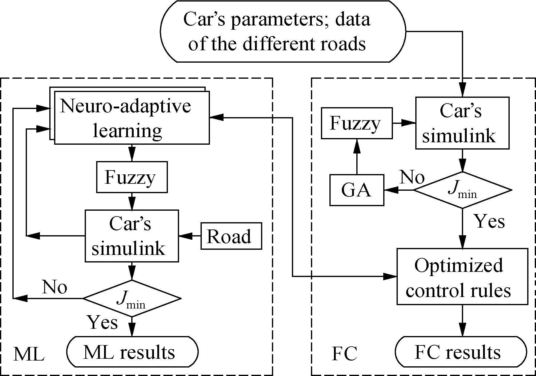
Fig.5 SAS control model combined with the FC and ML

(a)
(b)
(c)
Fig.6 Data map of the FC optimized control rules. (a) Soft road; (b) Rigid road; (c) Soft and rigid road
2.2 Control of ML from the FC control rules
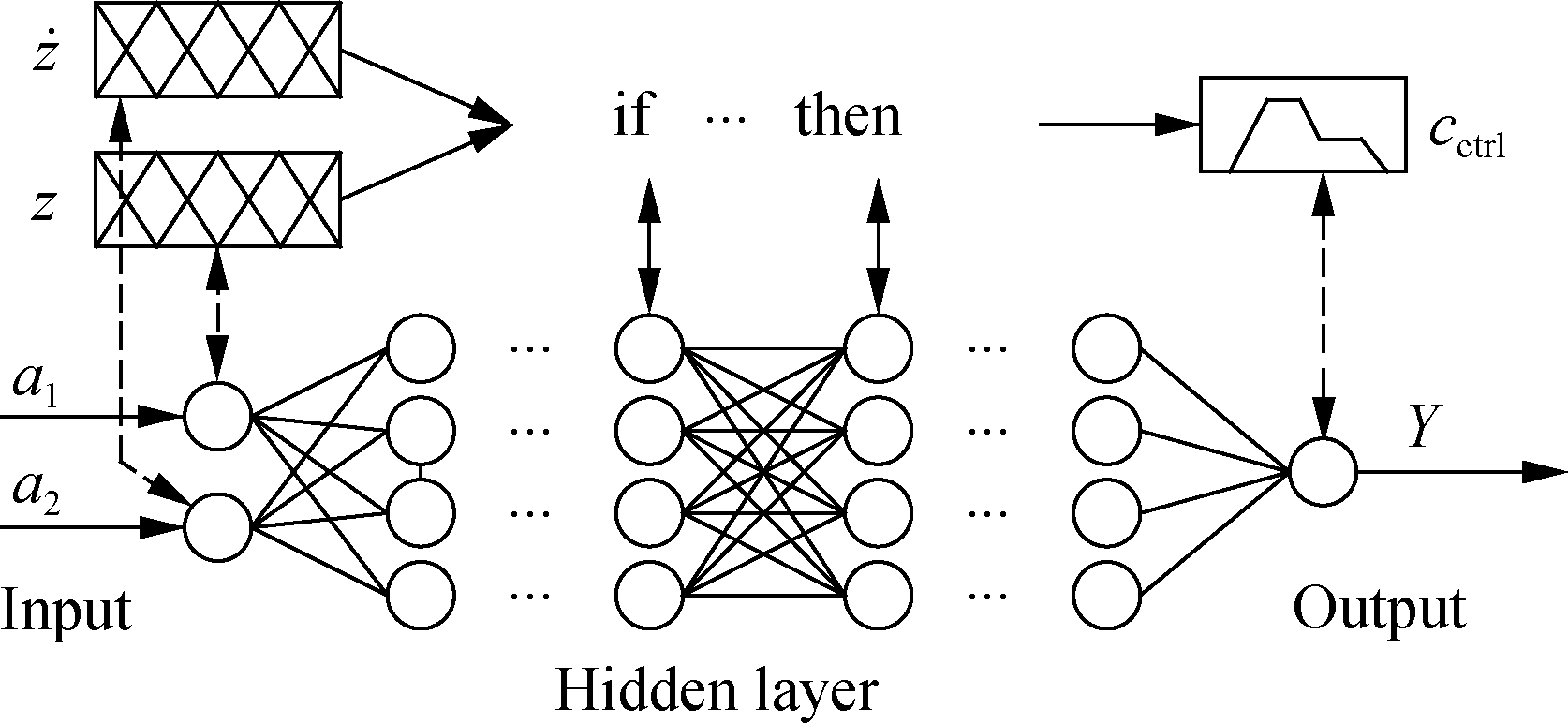
The FC efficiency optimized by the GA obtains the maximum value when the car is moving on a type of road surface. However, under a type of the actual road surface, the good, medium, and poor surfaces of the soft road or surfaces of ISO levels A, B, and C of the rigid road can concurrently appear on each surface of the soft and rigid roads when the car is moving. Thus, the optimized FC efficiency is reduced. Thus, from the data map of the FC control rules optimized on all the surfaces of the soft and rigid roads in Fig.6, neuro-adaptive learning in an adaptive neuro-fuzzy inference system (ANFIS)[12-13] was used to optimize the control efficiency of the SAS under various conditions of the car. The model of neuro-adaptive learning is provided in Fig.5 and labeled with “ML.”
The input signals n are defined by a vector of X={a1, a2,…, an}T, and the output signal Y of ML is computed by
(24)
where γis the trigger function; ϑi is the weight of ai; and α is the neural activation threshold.
Based on the ANFIS tool in the MATLAB software, a neuro-fuzzy controller (NFC) was then designed to learn all the optimized control rules of the data map, as shown in Fig. 6. The data of the input/output values of “z and
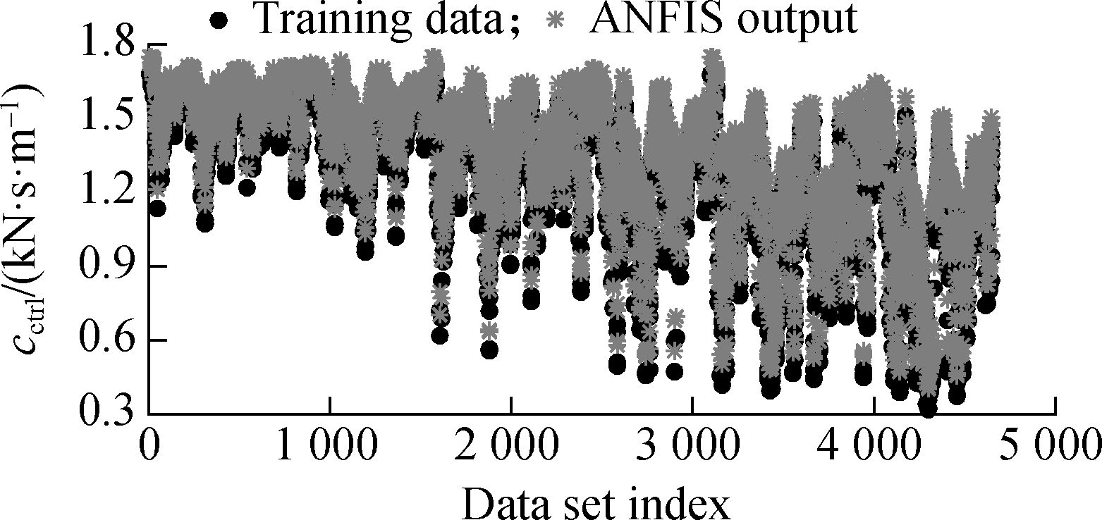
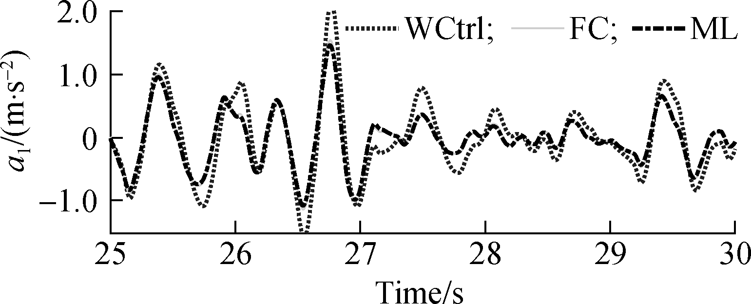
![]() and “cctrl” in MATLAB/workspaces were fed into the ANFIS via the input/output variables of “a1 and a2” and “Y.” The NFC model is plotted in Fig. 7(a). To perform the training process and ML in the ANFIS, the training method was chosen by Hybrid; the constituent rules’ number is three, comprising two input values and one output value; the training process error is 10-3; and the number of the training times is 103. The results of the training process are given in Fig. 7(b), and they are saved for the ML model to control cctrl of the SAS. The efficiency of the ML model was simulated and compared with the FC under the medium surface of the soft road and level B of the rigid road, as shown in Fig. 8.
and “cctrl” in MATLAB/workspaces were fed into the ANFIS via the input/output variables of “a1 and a2” and “Y.” The NFC model is plotted in Fig. 7(a). To perform the training process and ML in the ANFIS, the training method was chosen by Hybrid; the constituent rules’ number is three, comprising two input values and one output value; the training process error is 10-3; and the number of the training times is 103. The results of the training process are given in Fig. 7(b), and they are saved for the ML model to control cctrl of the SAS. The efficiency of the ML model was simulated and compared with the FC under the medium surface of the soft road and level B of the rigid road, as shown in Fig. 8.
(a)
(b)
Fig.7 ML model. (a) NFC model; (b) Training result of the NFC from the data map of the optimized control rules
(a)
(b)
Fig.8 Acceleration response of the driver’s seat. (a) Soft road; (b) Rigid road
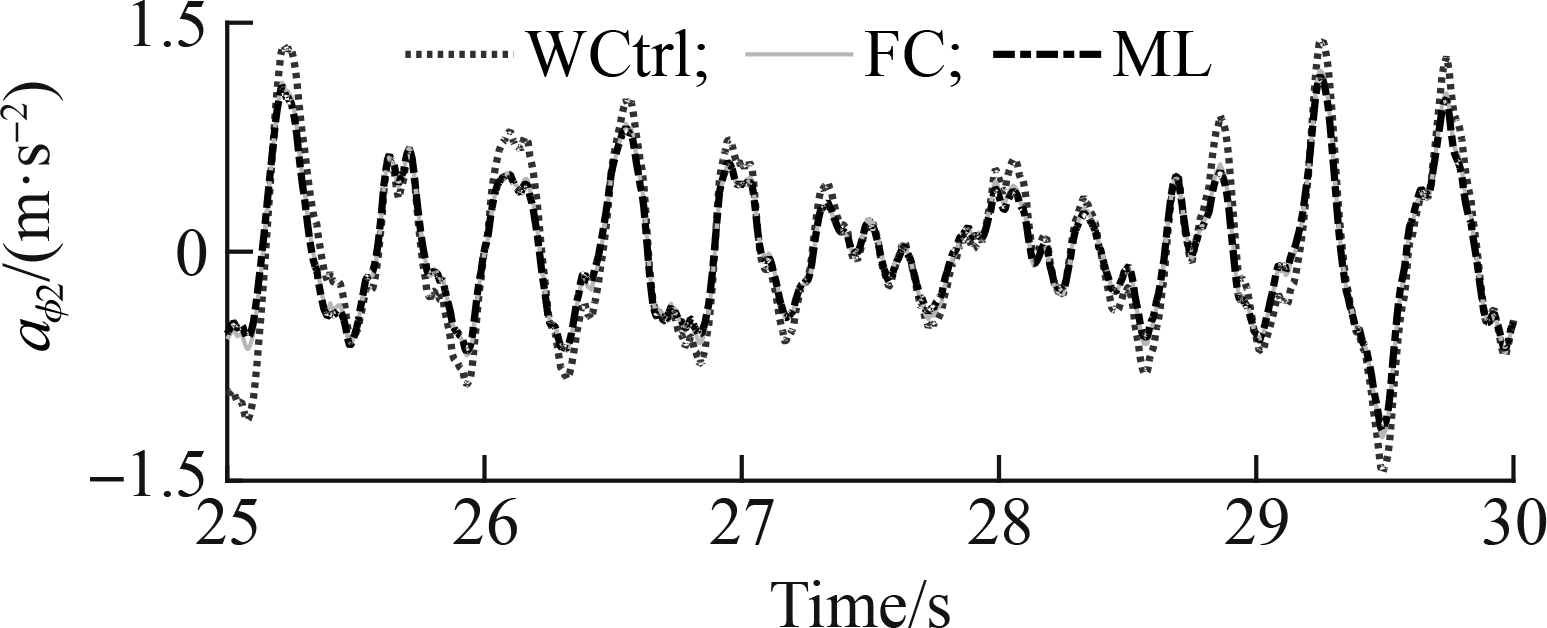
Fig. 8 shows that the acceleration response of the driver’s seat using the ML method is similar to the training data of the FC when the car is moving on a medium surface of the soft road or a rigid road surface of ISO level B. The calculation results in Tab. 4 indicate that the value of awz1 is slightly decreased by 0.57% on the medium surface of the soft road and 0.22% on the ISO level B of the rigid road surface. There is a small error between the FC and ML, which is due to a small error in the learning process of the ML. Moreover, the value of awz1 with the SAS is smaller than that without control (WCtrl) by 17.86% on the medium surface of the soft road and 20.64% on the ISO level B of the rigid road surface. Hence, the car’s ride quality with the SAS is improved. To evaluate the efficiency of the ML for the SAS, various moving conditions of the car were simulated and assessed.
Tab.4 Seat’s RMS acceleration

Control methodsawz1/(m·s-2)Soft roadRigid roadPassive0.646 20.555 2FC0.533 70.441 8ML0.530 70.440 8
3 Results and Analysis
3.1 Influence of soft road surfaces
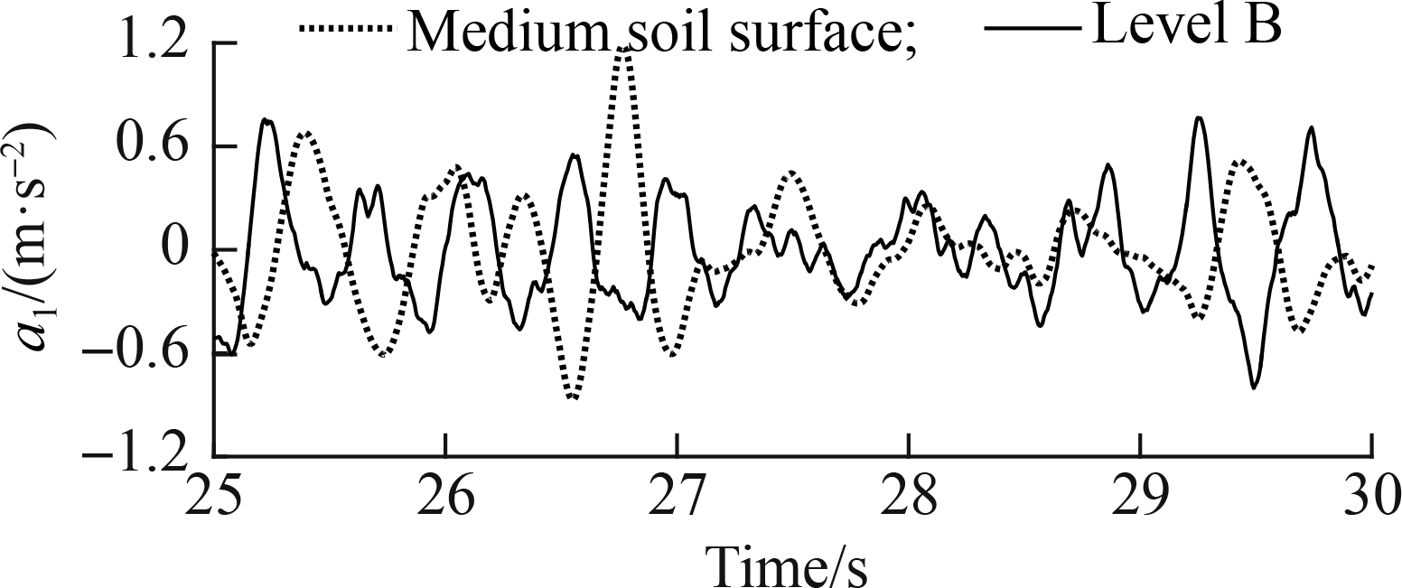
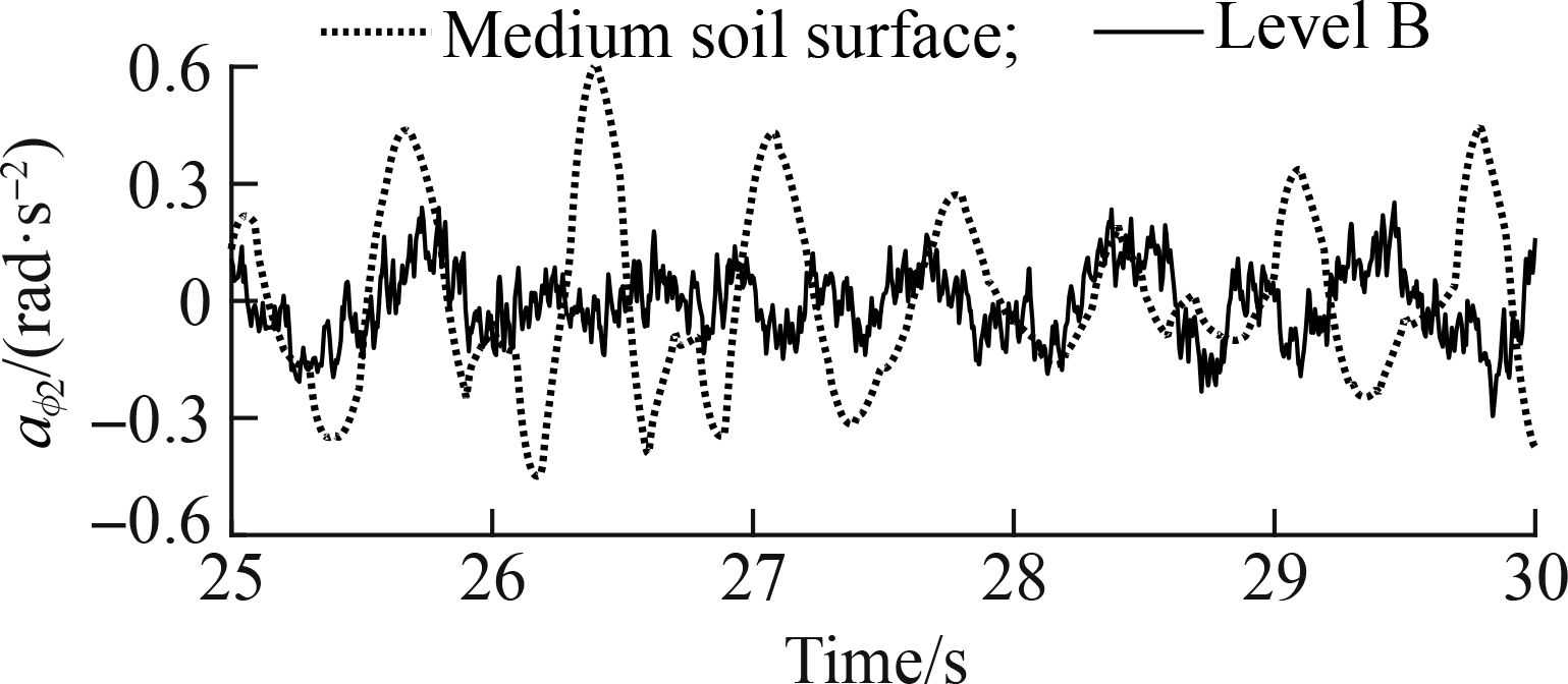
A car mostly moves on rigid road surfaces, so its ride quality is mainly evaluated under the excitation of different rigid road surfaces[5-6, 8]. However, in the same cases, the car can also move on soft road surfaces of the soil or sand grounds. Thus, soft road surfaces also affect the car’s ride quality and control efficiency of the suspension systems. However, this issue has not been evaluated yet in existing studies. To clarify this issue, a soft road with lumped parameters of n=1.01, kc=60 kN/mn+1, kφ=5 880 MN/mn+2, c=3.1 kPa, and φ=29.8o[17] of a medium surface was simulated and compared with the rigid road surface of ISO level B (medium level). The results of the acceleration responses and RMS values are provided in Fig. 9 and Tab. 5.
(a)
(b)
Fig.9 Acceleration responses under the medium level of the soft and rigid road surfaces. (a) Driver’s seat; (b) Car pitch
Tab.5 RMS accelerations under ISO level B of the rigid road and medium surface of the soft road

ParametersRigid roadSoft roadIncrease/%awz1 / (m·s-2)0.347 00.408 117.60awφ2/(rad·s-2)0.109 20.190 674.60
Fig. 9 indicates that under the same medium level of soft road and rigid road surfaces, the comparison results show that the accelerations of the vertical driver’s seat and car pitch angle on the soft road are higher than those on the rigid road. In particular, awz1 and awφ2 strongly increased by 17.60% and 74.60%, respectively. This outcome can be attributed to the effect of the deformable soil ground of the soft road under the impact of the static and dynamic loads of the wheels when the car is moving. Thus, the driver’s ride quality and car body’s shaking on the soft road were reduced in comparison with those on the rigid road. Hence, the soft road greatly reduces the driver’s ride quality and health in comparison with the rigid road.
3.2 ML efficiency for the SAS
Based on the ML result learned via the optimized FC rules, the ML efficiency has not been clearly demonstrated yet under the medium surface of a soft road or ISO level B of a rigid road in Section 2.2. Thus, a random road surface built from a combination of the poor-good-medium surfaces of the soft road, and a random road surface built from a combination of the ISO level C-level A-level B of the rigid road were applied to evaluate the ML efficiency as follows:

(25)

(26)
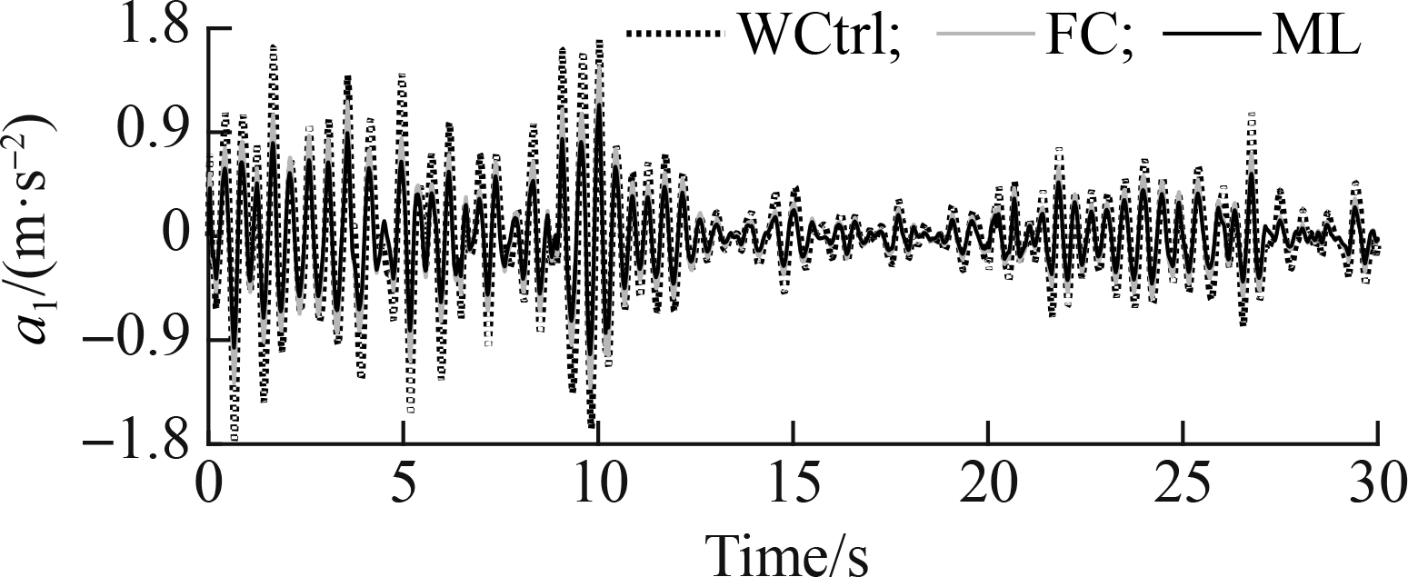
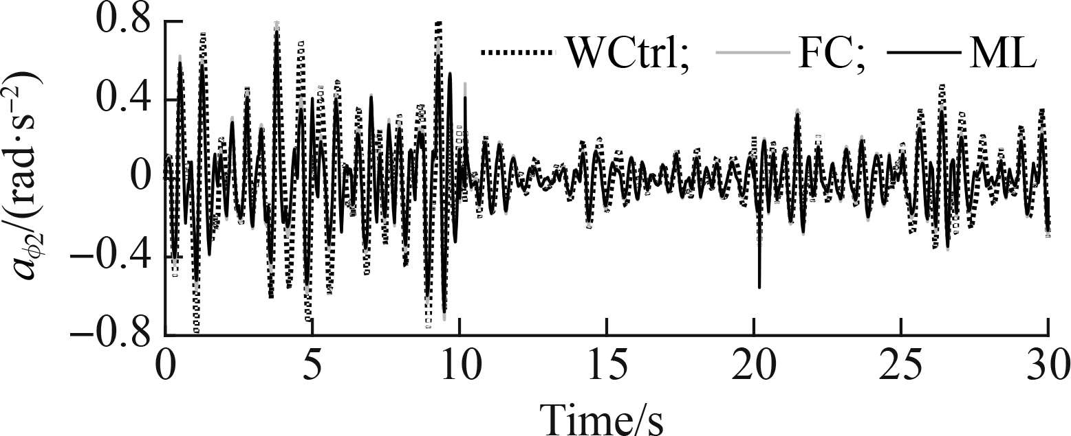
The acceleration responses of the driver’s seat and car’s pitch angle under the soft and rigid roads are shown in Figs. 10 and 11, respectively. Under the excitation of the poor-good-medium soil surface of the soft road, Fig. 10 shows that the accelerations of the driver’s seat and car’s body used in the ML model greatly decreased as compared to those of the FC and WCtrl. awz1 and awφ2 using the FC in Tab. 6 obviously reduced by 18.02% and 12.31% in comparison with those using the WCtrl, respectively, whereas awz1 and awφ2 using the ML model significantly decreased by 30.20% and 19.95% compared to those using the WCtrl, respectively. Thus, the control efficiency of the ML model is better than that of the FC.
(a)
(b)
Fig.10 Acceleration responses under the poor-good-medium surface of the soft road. (a) Driver’s seat; (b) Car pitch
Tab.6 Calculation results of the RMS accelerations

Road surfacesParametersWCtrlFCMLPoor-good-medium surface of the soft roadawz1/(m·s-2)0.607 50.498 00.424 0awϕ2/(rad·s-2)0.280 20.245 70.224 3Level C-level A-level B surface of the rigid roadawz1/(m·s-2)0.547 70.420 80.359 5awϕ2/(rad·s-2)0.175 00.151 70.137 1
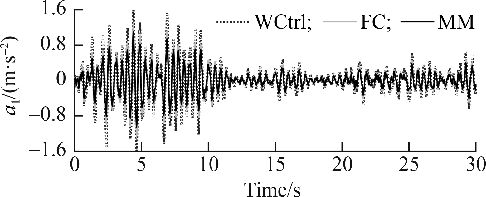
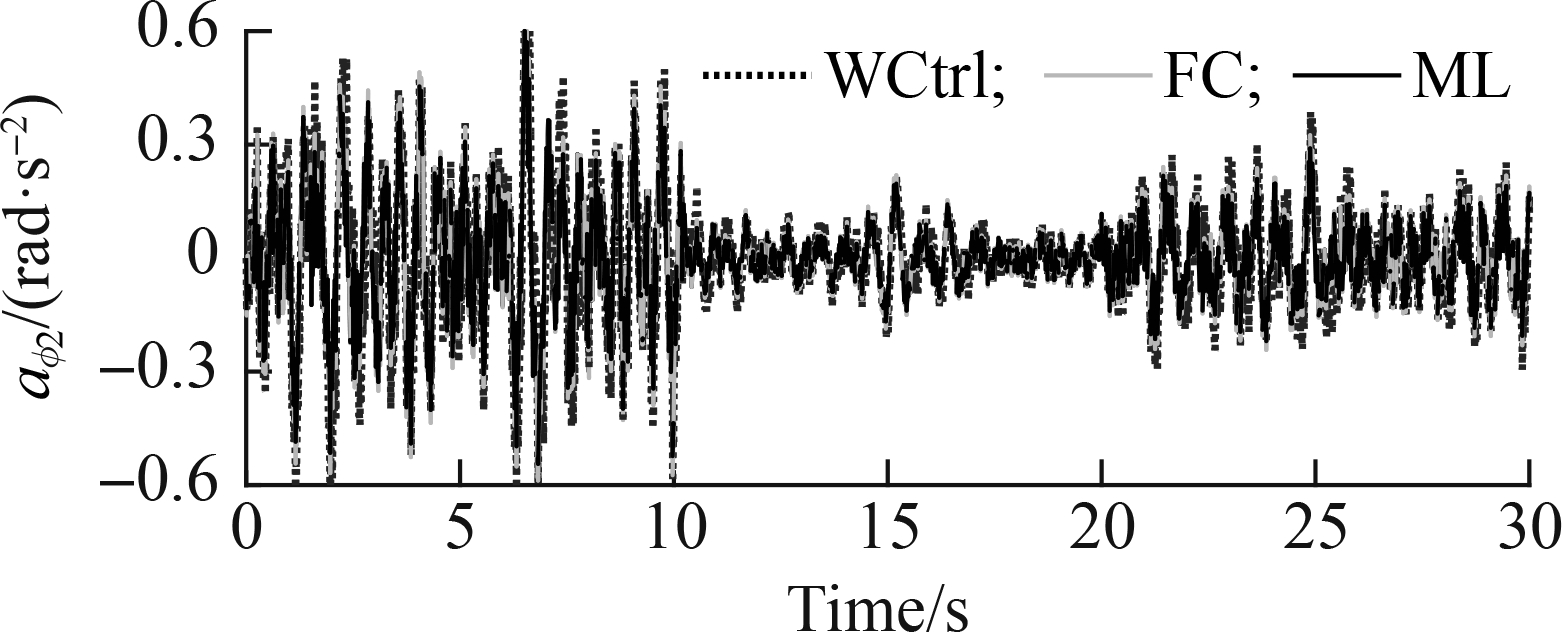
Similarly, under excitation of the ISO level C-level A-level B of a rigid road surface, Fig. 11 also shows that the accelerations of the driver’s seat and car’s body using the ML model are lower than those of the FC and WCtrl. The calculation results of awz1 and awφ2 with the ML model in Tab. 6 decreased by 34.36% and 21.66% in comparison with those using the WCtrl and by 14.56% and 9.62% compared with those using the FC, respectively. Therefore, the SAS controlled by the ML model can better improve the car’s ride quality in comparison with the FC under various excitations of the soft and rigid roads.
(a)
(b)
Fig.11 Acceleration responses under the level C-level A-level B surface of the rigid road. (a) Driver’s seat; (b) Car pitch
3.3 ML efficiency under different velocities
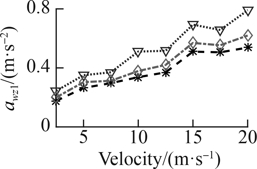
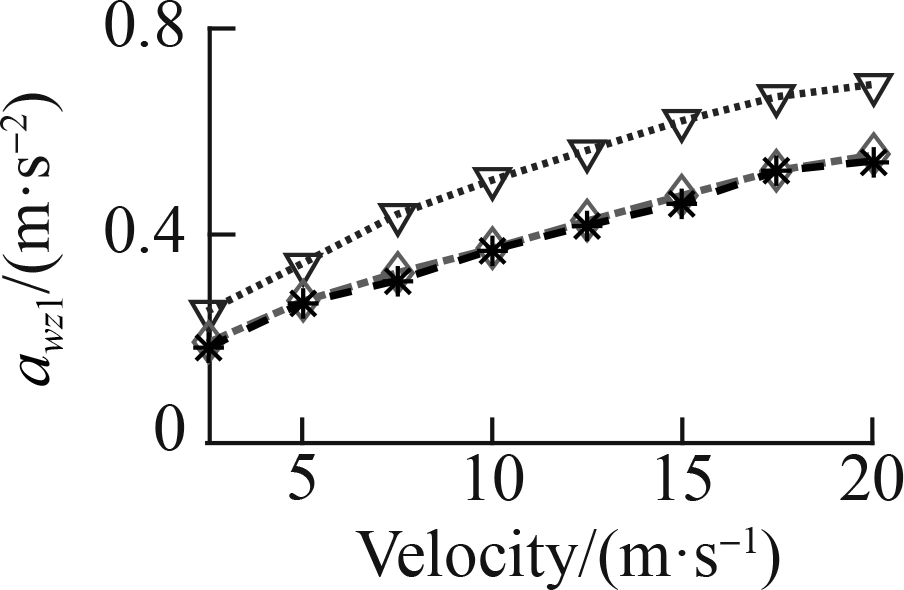
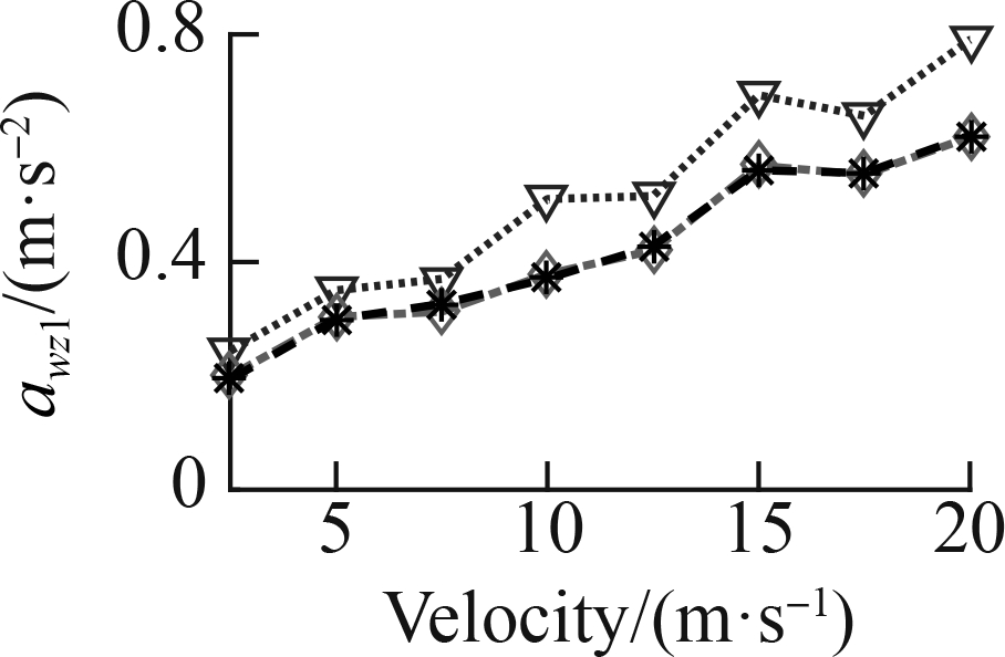
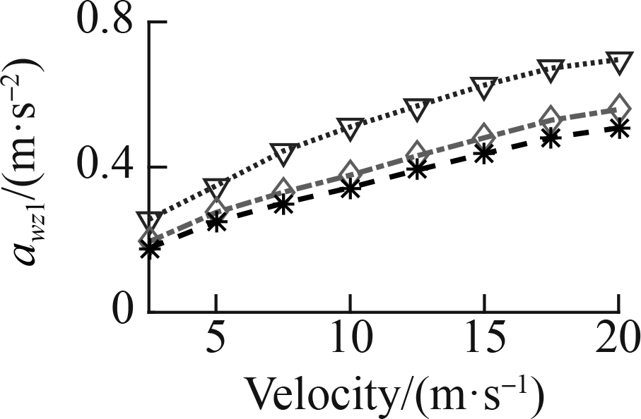
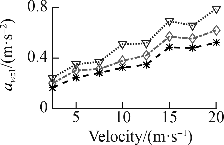
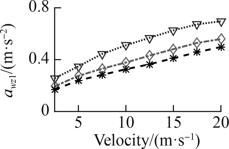
To fully assess the ML efficiency, a speed range from 2.5 to 20 m/s was also simulated in three cases: Case 1—the ML was only used by the data map of the soft road, Case 2—the ML was only used by the data map of the rigid road, and Case 3—the ML was used by the data map of the soft and rigid roads, as shown in Fig. 6. The awz1 results of the three cases are simulated and plotted in Fig.12.
(a)
(b)
(c)
(d)
(e)
(f)
Fig.12 RMS acceleration of the driver’s seat under various vehicle velocities. (a) Case 1 under soft road; (b) Case 1 under rigid road; (c) Case 2 under soft road; (d) Case 2 under rigid road; (e) Case 3 under soft road; (f) Case 3 under rigid road
Fig. 12(a) shows that under the influence of the soft road, awz1 quickly augmented, whereas Fig. 12(b) indicates that under the influence of the rigid road, awz1 insignificantly augmented, especially from 15 to 20 m/s. This result implies that the car’s traveling velocity needs to be limited when the car is traveling on a soft road. With the SAS controlled by the ML and FC, the result of awz1is greatly reduced compared to that in the WCtrl under the car’s different velocities on both the soft and rigid road surfaces. Therefore, the car’s ride quality is obviously ameliorated by the SAS.
In Case 1, with the ML model only using the data map of the soft road, Fig. 12(a) reveals that awz1 with the ML model is also significantly reduced in comparison with the FC under all the different velocities of the car traveling on the soft road. However, Fig. 12(b) reveals that awz1 with the ML model is insignificantly changed in comparison with the FC on the rigid road under the car’s different velocities. This result can be due to the ML learning process only learning the optimized control rules of the deformable surfaces of the soft road. Therefore, the ML control efficiency has been limited on the rigid road.
In Case 2, similarly, with the ML model only using the data map of the rigid road, the result of awz1 in Fig. 12(c) is unchanged on the soft road, whereas the result of awz1 in Fig. 12(d) is significantly decreased on the rigid road as compared to the result of awz1 controlled by the FC.
In Case 3, with the ML using the data map of the soft and rigid roads, both Figs. 12(e) and (f) indicate that the results of awz1 are obviously reduced compared to the FC under the car’s different velocities. Consequently, the car’s ride quality with the SAS controlled by the ML model is better than that of the FC. Concurrently, the ML control efficiency also depends on the learning data.
4 Conclusions
1) The deformable surface of soft roads greatly influences cars’ ride quality as compared to rigid roads under the same car simulation conditions. Therefore, cars’ velocities on soft roads need to be limited to assess their ride quality.
2) The ML efficiency for the SAS to assess a car’s ride quality is better than the efficiency of the FC and WCtrl under all the simulation conditions of the car. In particular, awz1 and awφ2 of the ML model were greatly reduced by 30.20% and 19.95% on the deformable surfaces and 34.36% and 21.66% on the rigid surfaces in comparison with the WCtrl, respectively.
3) The ML efficiency significantly depends on learning data. Thus, to optimize its efficiency, the map of the learning data for the ML model should be further expanded under various conditions.
4) The ML has not only learned the optimized control rules of the FC from the data map to further enhance the SAS control efficiency but also improves the car’s ride quality more than the FC under the combined different road surfaces.
[1] Wu M, Yin H, Li X, et al. A new dynamic stiffness model with hysteresis of air springs based on thermodynamics [J]. Journal of Sound and Vibration, 2021, 521: 116693. DOI: 10.1016/j.jsv.2021.116693.
[2] Yang L, Wang R C, Ding R K, et al. Investigation on the dynamic performance of a new semi-active hydro-pneumatic inerter-based suspension system with MPC control strategy[J].Mechanical Systems and Signal Processing, 2021, 154: 107569. DOI:10.1016/j.ymssp.2020.107569.
[3] Nguyen V, Jiao R Q, Zhang J R. Control performance of damping and air spring of heavy truck air suspension system with optimal fuzzy control[J].SAE International Journal of Vehicle Dynamics, Stability, and NVH, 2020, 4(2): 10-4. DOI:10.4271/10-04-02-0013.
[4] Fergani S, Sename O, Dugard L. A LPV/H∞ global chassis controller for performances improvement involving braking, suspension and steering systems[J]. IFAC Proceedings Volumes, 2012, 45(13): 363-368. DOI:10.3182/20120620-3-DK-2025.00169.
[5] Haemers M, Derammelaere S, Ionescu C M, et al. Proportional-integral state-feedback controller optimization for a full-car active suspension setup using a genetic algorithm[J].IFAC—PapersOnLine, 2018, 51(4): 1-6. DOI:10.1016/j.ifacol.2018.06.004.
[6] Yan G, Fang M X, Xu J. Analysis and experiment of time-delayed optimal control for vehicle suspension system[J].Journal of Sound and Vibration, 2019, 446: 144-158. DOI:10.1016/j.jsv.2019.01.015.
[7] International Organization for Standardization. Mechanical vibration-road surface profiles-reporting of measured data: ISO 8068[S]. Geneve, Switzerland: International Organization for Standardization, 1995.
[8] Nguyen V, Zhang J, Le V, et al. Performance analysis of air suspension system of heavy truck with semi-active fuzzy control [J]. Journal of Southeast University(English Edition), 2017, 33(2): 159-165.DOI:10.3969/j.issn. 1003-7985.2017.02.006.
[9] Nguyen V, Zhang J, Jiao R, et al. Effect of the off-road terrains on the ride quality of construction vehicles [J]. Journal of Southeast University(English Edition), 2019, 35(2): 191-197. DOI:10.3969/j.issn.1003-7985.2019.02.008.
[10] Mitschke M. Dynamik der Kraftfahrzeuge[M]. Berlin: Springer Berlin Heidelberg, 1972: 301-347.
[11] El-Sayegh Z, El-Gindy M, Johansson I, et al. Development and validation of off-road tire-gravelly soil interaction using advanced computational techniques[J].Journal of Terramechanics, 2020, 91: 45-51. DOI:10.1016/j.jterra.2020.05.004.
[12] Yuan H, Nguyen V, Zhou H X. Research on semi-active air suspensions of heavy trucks based on a combination of machine learning and optimal fuzzy control[J].SAE International Journal of Vehicle Dynamics, Stability, and NVH, 2021, 5(2): 10-5. DOI:10.4271/10-05-02-0011.
[13] Ye Y, Huang P, Zhang Y. Deep learning-based fault diagnostic network of high-speed train secondary suspension systems for immunity to track irregularities and wheel wear[J]. Railway Engineering Science, 2022, 30:96-116. DOI:10.1007/s40534-021-00252-z.
[14] Hua W L, Nguyen V, Zhou H X. Experimental investigation and vibration control of semi-active hydraulic-pneumatic mounts for vibratory roller cab[J]. SAE International Journal of Vehicle Dynamics, Stability, and NVH, 2021, 5(4): 10-5. DOI:10.4271/10-05-04-0028.
[15] Shi X M, Cai C S. Simulation of dynamic effects of vehicles on pavement using a 3D interaction model[J]. Journal of Transportation Engineering, 2009, 135(10): 736-744. DOI:10.1061/(asce)te.1943-5436.0000045.
[16] International Organization for Standardization. Mechanical vibration and shock—Evaluation of human exposure to whole body wibration—Part 1: General requirements: ISO 2631-1 [S]. Geneve, Switzerland: International Organization for Standardization, 1997.
[17] Wong Y J. Theory of ground vehicles[M]. New York, NY, USA: John Wiley & Sons, 2001: 145-198.