With the rapid increase in the demand for natural gas, supersized floating liquefied natural gas(FLNG)and liquefied natural gas carriers(LNGC)have been used as the most efficient tools for long-distance production and transportation of LNG at sea. Membrane tanks were the most widely used containers in these huge ships. They are made up of several invar membrane layers and insulation material, which can maintain the temperature of LNG around -110 K. However, the membrane tank was not a kind of high pressure vessel. When it is partially filled, the risk of sloshing impact and pressure variation should be considered. Sloshing of inner liquid was generally caused by ocean currents, waves and sea winds. When the excitation frequency from external forces was close to the natural frequency of the cargo containment system(CCS), a large amplitude sloshing could cause violent liquid movement and high-pressure impact on the tank shells. Therefore, an analysis of the sloshing phenomenon and free surface behavior in a FLNG tank is necessary.

Vessel motion was a classic problem in marine hydrodynamics, while solving the sloshing issue still remains a challenging task because many factors are involved, such as the type of disturbance, container shape and coupled problem with solid support. To investigate the modal characteristics, a modal analysis of both linearized and non-linearized free liquid surfaces in a rigid vessel was widely studied^[1]. However, analytical solutions^[2] were limited to regular geometric tank shapes, such as cylinders or rectangles. Then, an approximate analytical solution for more structures was developed by Evans. For many engineering problems, Yakimov et al.^[3] proposed a simple and quick method to calculate nonlinear one-dimensional and three-dimensional boundary problems. A new method using operator equations for periodic gravity waves on water of finite depth was derived by Dinvay et al^[4]. Numerical methods were widely used to decribe the fluid sloshing based on finite element simulation. Based on the small displacement assumption, an irrotational fluid can be modeled by a degenerate solid finite element^[5], which was introduced using commercial ANSYS code to simulate the sloshing problems in engineering fields.

Due to the fast development of computer capacity, numerical simulation is becoming a promising tool for studying fluid sloshing. It can not only accurately locate the natural frequency of some complex vessels, but also describe the free surface motion inside these structures. At first, grid-based methods were applied to represent a submerged hydrofoil with a fully nonlinear free surface^[6], which resulted in a highly accurate free surface compared with experiments. However, due to the grid restriction, when numerical simulation was used to decribe the free surface with large deformations or those quickly changing, refreshing the grids to fit the violent free surfaces is very computationally expensive. The grid-free method was required in the calculation of the interface between liquids and gases. The smoothed particle hydrodynamics(SPH)method replaced the physical objects with a set of particles that have individual masses. By solving the governing equations according to the SPH algorithm^[7], Shamsoddini et al.^[8] investigated the pressure on solid boundaries in a 2D sloshing problem using an improved SPH method, and obtained a good agreement with the experiment. Another numerical method used for unsteady Navier-Stokes equations was the level-set method, which was usually used in handling merging, breaking and self-intersecting interfaces in violent-free surface motion^[9]. The volume-of-fluid(VOF)method was based on the concept of a fractional volume of fluid, which was shown to be more flexible and efficient for treating complicated free configurations^[10]. Kim^[11] used the SOLA-VOF method to simulate the liquid sloshing in a 2D container. A special buffer zone was adopted near the tank ceiling to affect the impulsive pressure, and a single-value function was used to track the sloshing interface. Lu et al.^[12] applied a viscous fluid model based on the non-inertial reference system to study the liquid sloshing in rectangular tanks with or without baffle. The sloshing responses was reported to be finally dampened due to the physical dissipations, which were greater in baffled tanks. Li et al.^[13] used the VOF method and OpenFOAM software to analyze the sloshing behavior in a baffled FLNG tank, which was separated into two main spaces. The moment of liquid impact force was compared under different filling rates. Their work indicated that the baffled tank can increase the energy loss of sloshing liquid, but decrease the sloshing amplitude. To obtain a better understanding of the sloshing tank under natural frequencies, Kawahashi et al.^[14] did experimental and numerical research at the near-natural frequency. The coupled influence of outside stimulating motions and internal liquid sloshing was studied. Sway and roll motions had a more significant effect on the partially filled tank. Therefore, roll motion was selected as the tank motion in this work. Additionally, the natural frequency and amplitude were highly dependent on the baffle width and position. Due to the fast computational time and the accurate description of the free surface, the VOF method has become a more popular tool.

In general, a comprehensive investigation was conducted for the sloshing problem in rectangular tanks. However, several aspects associated with the sloped bottom required further clarification for the design and operation of FLNG membrane tanks, such as the influence of the sloped bottom on the sloshing response and the magnitude of the pressure loading on the wall. These issues will be studied in this work using numerical simulations by the VOF method. 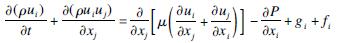After verifications and validations against experimental and other numerical data, the liquid response around the lowest natural sloshing frequency will be studied in different sloped-bottom tanks.

Mass and momentum conservation equations of an incompressible fluid in a non-inertial reference system can be written as follows:

Continuity equation

(1)

Momentum equation

(2)

where x_i is the coordinate; ρ is the density; P is the pressure; u_i, g_i and f_i are the velocity, gravitational acceleration and body force terms in the i-th direction, respectively. Body force term f_i is the acceleration of the non-inertial coordinate system with respect to the ground.

The turbulence is modeled using the standard k-ε turbulence model, which has been extensively used for industrial applications. In addition, the standard k-ε turbulence model is more economical in terms of computational time^[15]. The turbulent viscosity μ_t is given as

μ_t=c_μρ(k²)/(ε)(3)

where c_μ is a practical constant of the standard k-ε model.

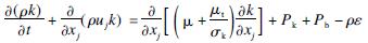
The turbulent kinetic energy equation(k)is

(4)

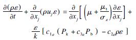
and the dissipation rate of the turbulent kinetic energy(ε)is

(5)

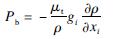
where μ is the viscosity of fluid; P_k represents the generation of turbulence kinetic energy due to the mean velocity gradients; and P_b is the generation of turbulence kinetic energy due to buoyancy, which are defined as

(8)

The constants used in the standard k-ε turbulence model are given as^[16]

σ_k=1.0, σ_ε=1.3, c_1ε=1.44

c_2ε=1.92, c_3ε=0.09, c_μ=0.09(9)

For free surface simulations, the VOF method is applied by the commercially available computational fluid dynamics(CFD)package FLOW-3D. The software utilizes the Hirt-Nichols' VOF method to compute the free surface motion. This model is suitable for tracking the interface with a low overall contact area and can provide a smooth surface. Surface tracking involves three processes: locating the interface, defining a sharp interface between the liquid and air, and setting boundary conditions at the interface. In the sloshing tank, the interface between the water and air is computed by solving the following equation:

(10)

where S₂ is the source of the gas, which equals zero in the tank; and α₂ and ρ₂ represent the volume fraction and density of the gas, respectively. The volume fraction of the liquid phase(α₁=V₁/V)is obtained as

α₁=1-α₂(11)

In later simulations, the free surface is represented by setting the water volume fraction to be 0.5, which implies that a grid cell is filled with 50% water and 50% gas. All grid cells over this value indicate the volume of water and the shape of the liquid-gas interface formed, which corresponds to the free surface.

Based on the viscous fluid theory, a non-slip wall condition is applied on the solid wall, and the fluid immediately next to the wall assumes the velocity of the wall. The Courant number is typically used to limit the time step size and should not be larger than 1 for numerical stability. However, in implicit unsteady simulations, the time step is controlled by the flow properties rather than the Courant number. To balance the computational accuracy and running time, the initial time step was set to be 0.01 s and automatically controlled by the stability and convergence of the pressure. The maximum number of pressure iterations before the time step is reduced to 50.

Additionally, the proper initial conditions should be followed. Filling height in previous studies is fixed at 5.36 m. The sloshing amplitude is 1° and starts from the horizontal position. All of these boundary conditions are with respect to the non-inertial coordinate system, as shown in Fig.1. The inertial coordinate system XYZ is fixed on the ground and the non-inertial system xyz rotates simultaneously with the tank. These two coordinate systems share the same z-axis, which is also the rotating axis of the tank. The position of a particle in the XYZ system is located at vector position(r(t),θ(t))and in the xyz system, and the position is(r(t),θ'(t)). Then, the angular position of a particle in the XYZ system can be written as

θ'(t)=θ(t)-Φt(12)

where Φ is the angular rate of the XYZ system. As the origin points of the two system are the same, the radial distance remains the same. Then, when the angular rate of the tank's rotation is set the same as the rotation of the XYZ system, which implies dθ/dt=Φ, the tank position in the non-inertial system xyz will remain unchanged, which is very helpful in the post-process of free surface description.

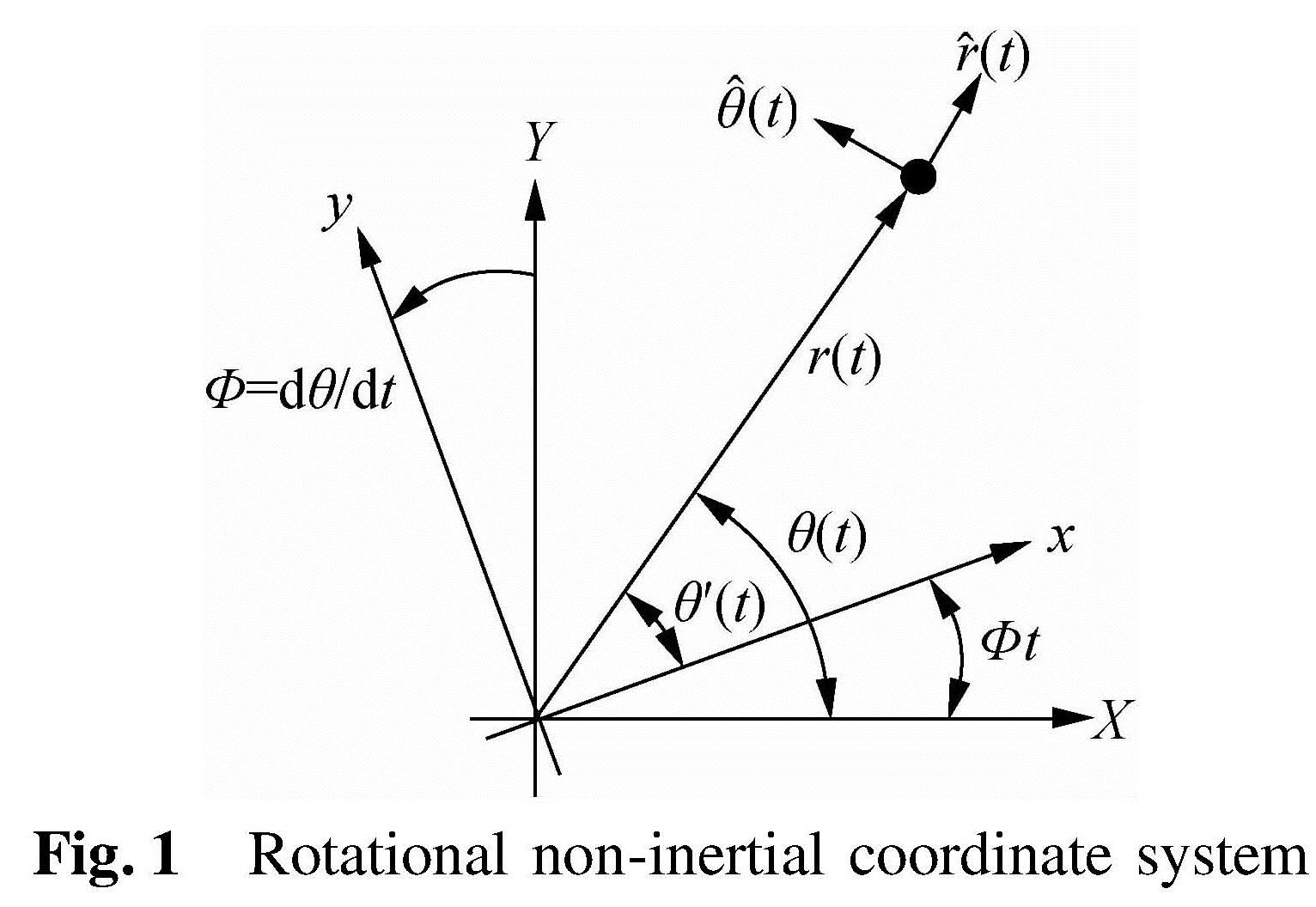
Fig.1 Rotational non-inertial coordinate system

Liquid material in the following study is simplified into liquid methane, which occupies 80%to 99% in the LNG mixture. The properties of liquid methane are listed in Tab.1.

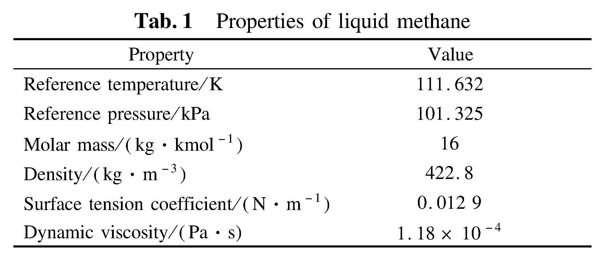
Tab.1 Properties of liquid methane

The geometric size of the sloshing tank is selected based on a real FLNG membrane tank^[17]. The inner width is 37.9 m and the height is 26.8 m, as shown in Fig.2. As this work focuses on the sloshing within the sketch plane, the stretch length is reduced to 2.4 m to save computing time. In addition to the geometry simplification, there should be sloped structures near both the ceiling and bottom in a real membrane tank. However, according to the previous study^[18], a sloped top helps liquid split from the side wall and results in a more violent surface behavior. Therefore, in this sloped-bottom investigation, the tank roof is simplified into a right angle.

The free gridding method used in the FLOW-3D software package is different from other computational fluid dynamic algorithms. In free gridding, geometry building operations and grid generation are independent of each other. The software is free to modify either the grid or the geometry without rebuilding the other. Therefore, this makes FLOW-3D a highly efficient software package to solve free surface problems. In this model, the entire computational domain is defined as a parameterized rectangular grid system. Every hexahedral cell is assigned one of five conditions: solid, part solid and part fluid, completely fluid, part fluid and part empty, and completely empty. As shown in Fig.2, dashed lines are the boundary of the whole grid system. The area filled with a green slash is left for the sloshing of the tank, which is initialized as the empty zone. Then, the solid geometry is placed using the fractional area volume obstacle representation(FAVOR^TM)method, which is represented by the gray area in the sketch.

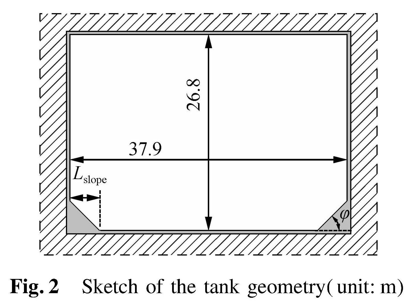
Fig.2 Sketch of the tank geometry(unit:m)

As the grid method in FLOW-3D does not consider the shape of liquid surfaces, curved cavities or other structures, the key for reducing the stair-stepping effect is the quantity of variably sized hexahedral cells, which are commonly associated with rectangular grids^[19]. As expected, more grids should produce a smoother numerical liquid surface, but this inevitably requires more calculation resources. Therefore, there is a minimum grid quantity that can provide a usable surface result. A grid independence study is implemented to determine the minimum number of cells required for sloshing problems in a FLNG-sized tank. Here, the slope angle Φ is set to be 0°.

Six simulation cases with different grid quantities(Case 1: 0.1×10⁶; Case 2: 0.2×10⁶; Case 3: 0.5×10⁶; Case 4: 1.0×10⁶; Case 5: 1.5×10⁶; Case 6: 2.0×10⁶)are carried out for the same sloshing condition. The time historical surface elevation at the symmetric middle position is shown in Fig.3. The patterns developed by all six cases are similar to a sinusoid with a growing amplitude. However, in the enlarged view of the local peak value, there are some elevation differences in each case. Three cases with smaller grid quantities provide relatively smaller peak values; however, the other three cases result in larger peak elevations. To show the difference caused by grid quantity, the historical development of the surface elevation is compared between paired cases, as shown in Fig.4. The greatest difference is approximately 0.84 m, which is unacceptable in the surface behavior study. However, by increasing the grid number, this difference is significantly reduced. When comparing Case 4 with Case 5 and Case 5 with Case 6, the greatest differences are only 0.082 and 0.061 m, respectively. The average elevation difference is dramatically reduced when the grid quantity is greater than 1.0×10⁶, which is only 0.024 m. Therefore, the grid model in Case 4 is selected as the optimum one.

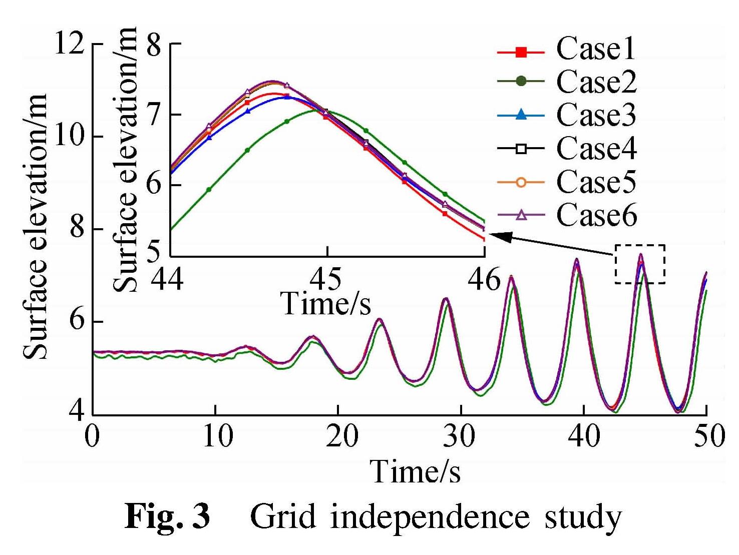
Fig.3 Grid independence study

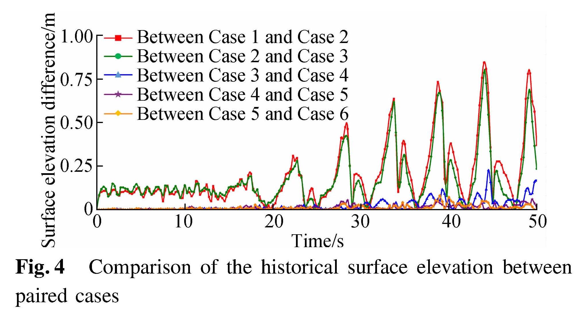
Fig.4 Comparison of the historical surface elevation between paired cases

In this section, simulation of water sloshing in a rectangular tank is used to validate the developed VOF model. According to Lee et al.^[20], sloshing in the IMO B type LNGC containment system is a typical nonlinear impact structural response. A pressure-impulse diagram for the self-supporting prismatic-shape tank should be studied and it can be useful for the damage-tolerant design of cargo tanks. Therefore, pressure impulse and liquid shape from the numerical result will be compared with the experimental data and the simulation from the SPH method by Chen et al^[21]. The geometry size of the tank is 1.0 m in width and 1.0 m in height with a water depth of 0.3 m. An rotational axis is set at the center of the tank bottom. The rolling amplitude is 5° and the excitation frequency is 3.81 rad/s.

Fig.5 gives the time histories of pressure on the left wall. The monitoring point is 0.1 m apart from the bottom. All three cases share a very similar cycle length. Although some differences appear in the 3rd and 4th peak values, the oscillation tendency of this model agrees well with Chen's experimental and SPH numerical results. Fig.6 and Fig.7 show qualitative behavior when the tank rotates to the edge and the horizontal positions. At the moment of 1.75 cycles, water is thrown to the highest position on the boundary walls. At the moment of 2.0 cycles, it moves in the maximum velocity from one side to the other. This pattern is repeated in all three cases, which means that the developed VOF model is qualified to describe the liquid sloshing in this kind of container.

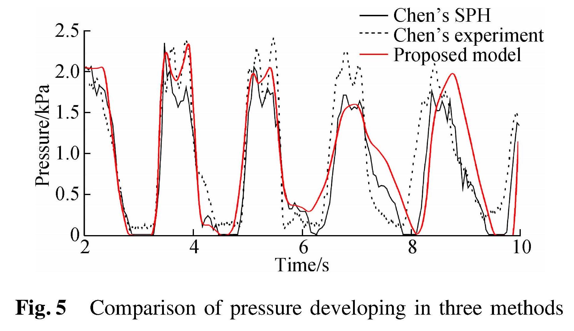
Fig.5 Comparison of pressure developing in three methods

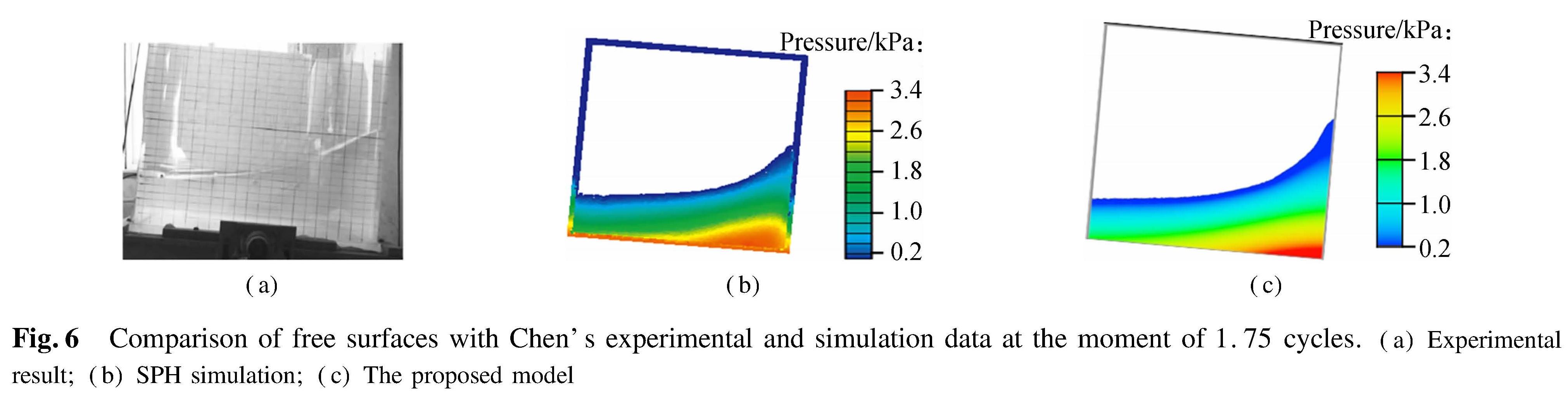
Fig.6 Comparison of free surfaces with Chen's experimental and simulation data at the moment of 1.75 cycles.(a)Experimental result;(b)SPH simulation;(c)The proposed model

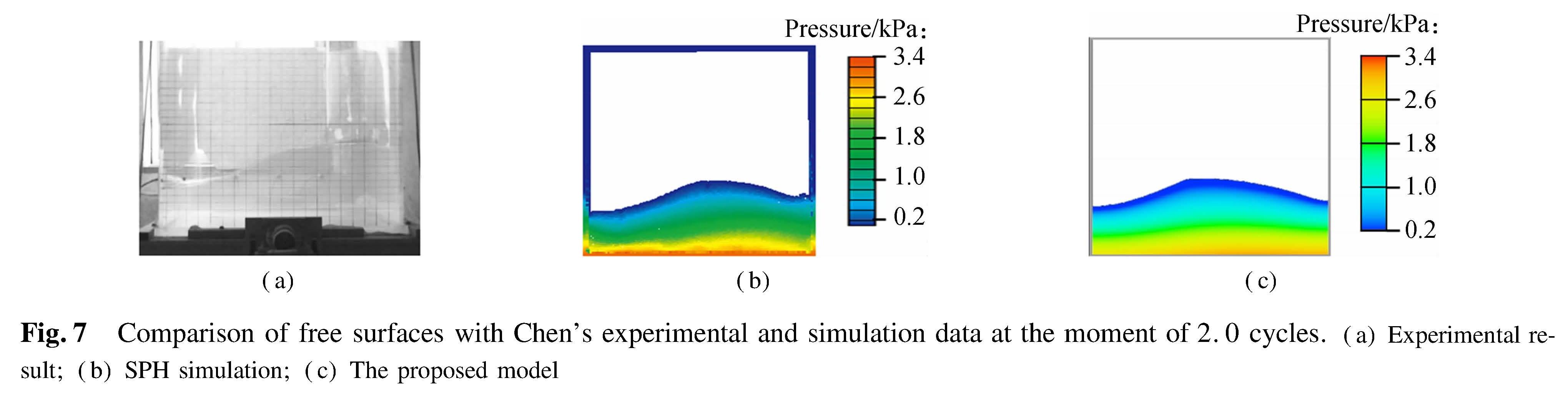
Fig.7 Comparison of free surfaces with Chen's experimental and simulation data at the moment of 2.0 cycles.(a)Experimental result;(b)SPH simulation;(c)The proposed model

Normally,the natural frequency of sloshing is calculated by the geometry size of the container, such as the wet length method and approximate analytical solution. In the first calculation method, the wet length is defined as the length of sloped bottom under water. Then, the natural frequency of a sloped-bottom tank is related to a rectangular tank with a projected bottom length.

The calculation of a rectangular tank is

ω²₀=(gπ)/(L)tanh(πh)/(L)(13)

By projecting the wet length to the bottom, the natural frequency in the wet length method is

ω²₀=(gπ)/(L/cosφ)tanh(πh)/(L/cosφ)(14)

The approximate analytical solution uses another strategy. The lowest natural frequency is calculated as

where x is the horizontal axis; y is the vertical axis; Ω is the area occupied by the liquid, and the original point of this coordinate is located in the middle of the initial liquid surface.

This kind of theoretical method has proved helpful in regular containers, for instance, rectangular tanks and cylinder tanks. However, if the container has some addictive structures, the calculation will come out with different results, as shown in Fig.8. As the bottom slope grows larger, the calculated natural frequency of the wet length method shows a dramatical decrease, but the calculated result of the approximate analytical solution only has

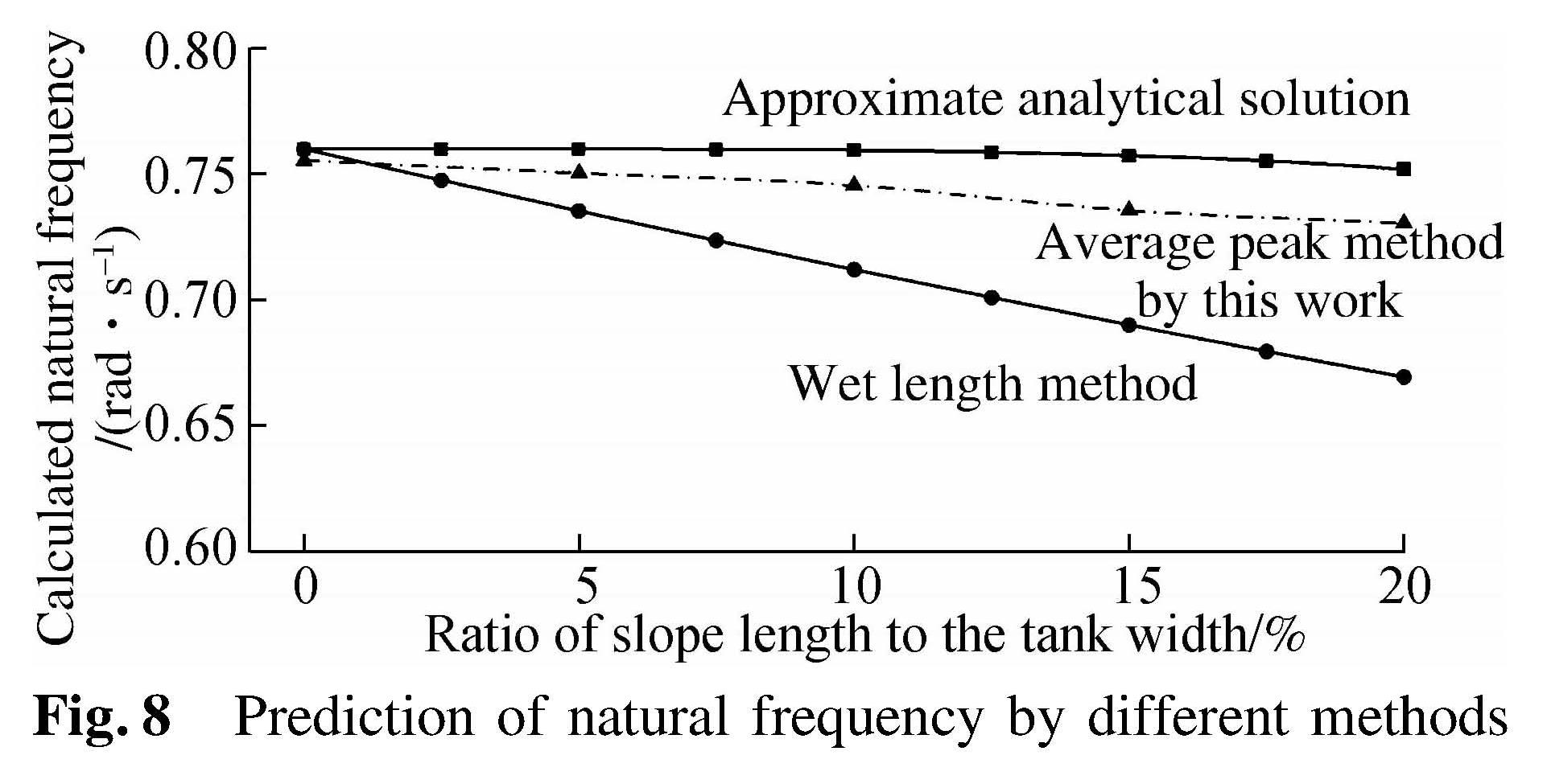
Fig.8 Prediction of natural frequency by different methods)

a small decline. These two results confuse researchers. Therefore, more accurate methods need to be developed.

The surface behavior under the natural frequency is much more violent than that under other excitations. Therefore, the natural frequency can be located by comparing the violence of liquid sloshing. Usually, the average or peak value of hydrodynamic parameters, such as pressure and fluid elevation, are directly utilized to evaluate the liquid behavior. For example, in the latest work from Zhao et al.^[22], the peak value of liquid amplitude was applied to define the natural frequency of two-combined FLNG tanks, which is taken as the worst condition in later simulations. Also, Sun et al.^[23] used the maximum of pitching RAOs(rad/m)as the single value to locate the natural frequency and study the shift of this frequency at a different filling rate(η). However, similar to our former study^[24], the accuracy of the evaluation might be affected by the container shape or using an inappropriate time duration. Our team proposed an improved average peak method to quantize the liquid behavior.

Firstly, the original data is obtained from the simulation results. Then, the graphic sloshing is described by some hydrodynamic parameters. To process this data, an automatic procedure is designed in the Matlab software package to find the single peak value during one sloshing period. By calculating the average of all these peak values in the same excitation, the comparison can be done to find the most violent situation corresponding to the natural frequency. In addition, some deeper analysis such as the frequency domain can also be done in this procedure.

The regular tank without a slope bottom is applied to validate the average peak method. 40% filling rate is used in the geometry model, as shown in Fig.2. The natural frequency in the two theoretical methods are both 0.76 rad/s. As shown in Fig.9(a), the excitation frequency of 0.75 rad/s leads to the largest average peak pressure on the side wall and decreases in both two directions. This response pattern is a typical natural frequency situation, which is very close to the natural frequency of 0.76 rad/s from theoretical methods.

However, when the ratio of slope length to tank width(γ)increases to 20%, theoretical methods give different predictions, as shown in Fig.9(c). According to the wet length method, the calculated natural frequency of this structure(γ=20%)is 0.67 rad/s. The corresponding average peak pressure is 13.24 kPa, which only accounts for 37.5% of the calculated pressure by the average peak method(35.35 kPa). This difference indicates that the calculation result from the wet length method is far from the most violent sloshing and the excitation here is not the expected one. Similar to the approximate analytical solution and the simplified rectangular tank without slope structure, their calculations deviate from the largest pressure. The pressure drops are 7.01 and 12.08 kPa, respectively. Therefore, the average peak method is considered more suitable for calculating the natural frequency in such complicated containers.

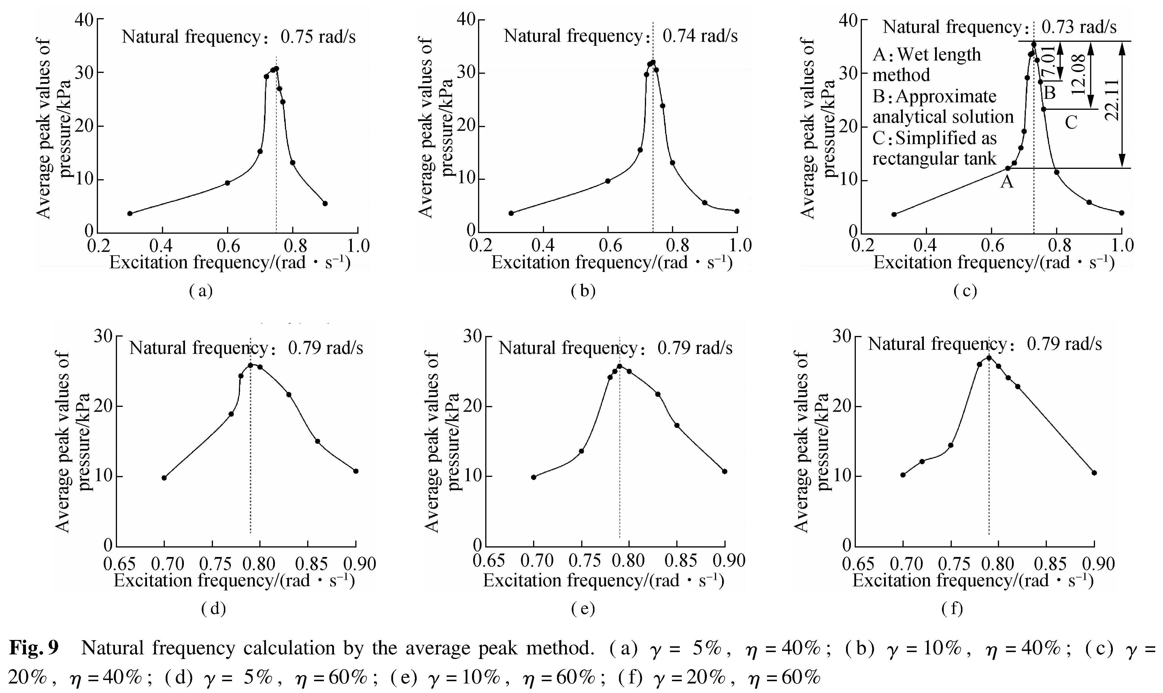
Fig.9 Natural frequency calculation by the average peak method.(a)γ= 5%, η=40%;(b)γ=10%, η=40%;(c)γ= 20%, η=40%;(d)γ= 5%, η=60%;(e)γ=10%, η=60%;(f)γ=20%, η=60%

To investigate the influence of the slope size on natural frequency, different slope structures are studied in this section. γ is set to be 0%, 10% and 20%, respectively. The frequency responses in two filling rates(η=40%, η=60%)are shown in Fig.9. With a lower filling rate of 40%, the natural frequency decreases gradually with the increase in the slope size. In the tank, with the largest slope, the natural frequency drops from 0.75 rad/s(rectangular tank)to 0.73 rad/s. However, with a higher filling rate of 60%, the natural frequency is very stable and keeps at 0.79 rad/s. This means that enlarging the slope will lower the natural frequency, but the connection is only obvious with a small filling rate. If the filling rate is high enough, the influence will be dampened.

As the natural frequency for each structure can be precisely located by the average peak method, comparison in this part will be proceeded under the most violent condition, respectively. First, the filling rate of 40% is applied to four tanks with different slope structures. Differently from previous studies, the excitation frequency in these four screenshots are set to be their own natural frequency, which may not be the same. Fig.10 gives the liquid position when the largest historical pressure occurs. This moment is not when fluid goes to the largest elevation, but when the highest velocity near the wall appears. According to the former study, the tank position at this moment is horizontal. Next, the worst situation can be analyzed.

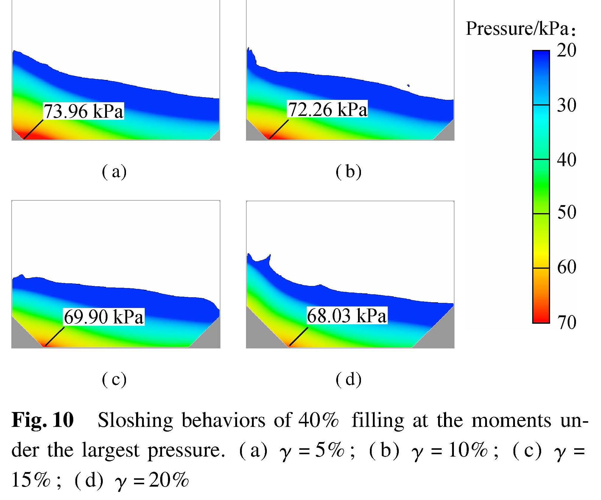
Fig.10 Sloshing behaviors of 40% filling at the moments under the largest pressure.(a)γ=5%;(b)γ=10%;(c)γ=15%;(d)γ=20%

It is found that in all four graphs, the highest pressure is always near the bottom corner, which is not the usual monitoring location on the side-wall. As the majority of fluid flows to the other side, the high pressure area will move in the meantime, but the local peak pressure will be smaller. So, the peak pressure in these graphs is not only the area peak value, but also the time historical one. From the area of high pressure, it can be found that the tank with the smaller slope comes with a bigger high pressure area, which will increase the affected area on the solid layers. When the slope size increases, the affected area will decrease quickly. Another decreasing parameter is the peak value of pressure, as shown in Fig.11. The average peak pressure decreases by 5.45 kPa when the ratio of slope length to tank width increases from 5% to 20%(7.4% to the highest one). The decreasing process is nearly linear, which means that slope size plays an important role in this filling condition and can improve the pressure loading on wall boundaries.

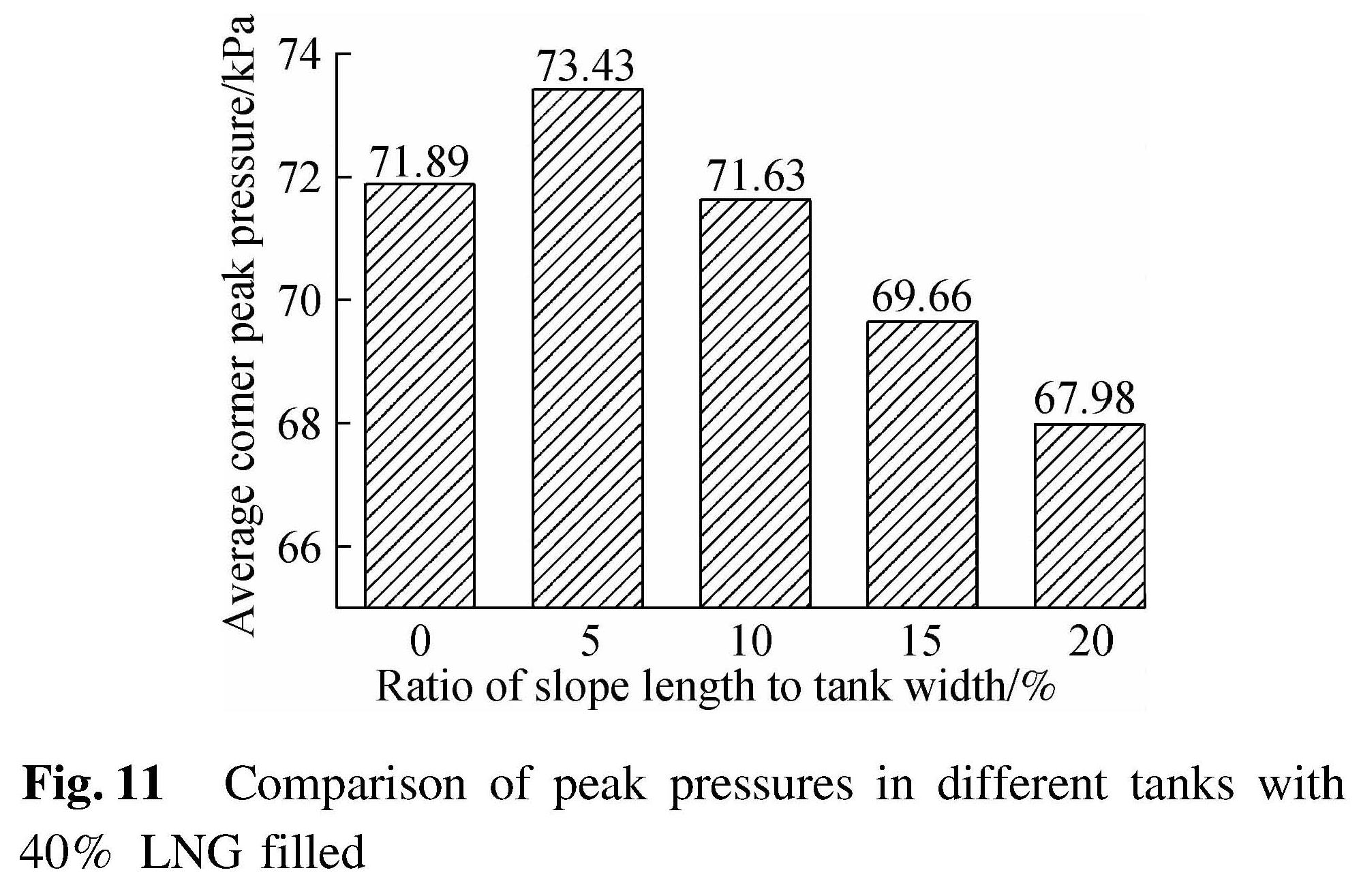
Fig.11 Comparison of peak pressures in different tanks with 40% LNG filled

However, when the filling rate becomes higher, this affected pattern shows some differences. The same part with the 40% filling rate is the high pressure area, shrinking with the increase in the slope length, as shown in Fig.12. However, the peak pressures in four violent moments have a different response tendency. As shown in Fig.13, the variation range of the pressure is only 1.35 kPa, which is about 1.6% of the highest one. In addition, the changing pattern here is no longer a continuous decrease but a more stable one.

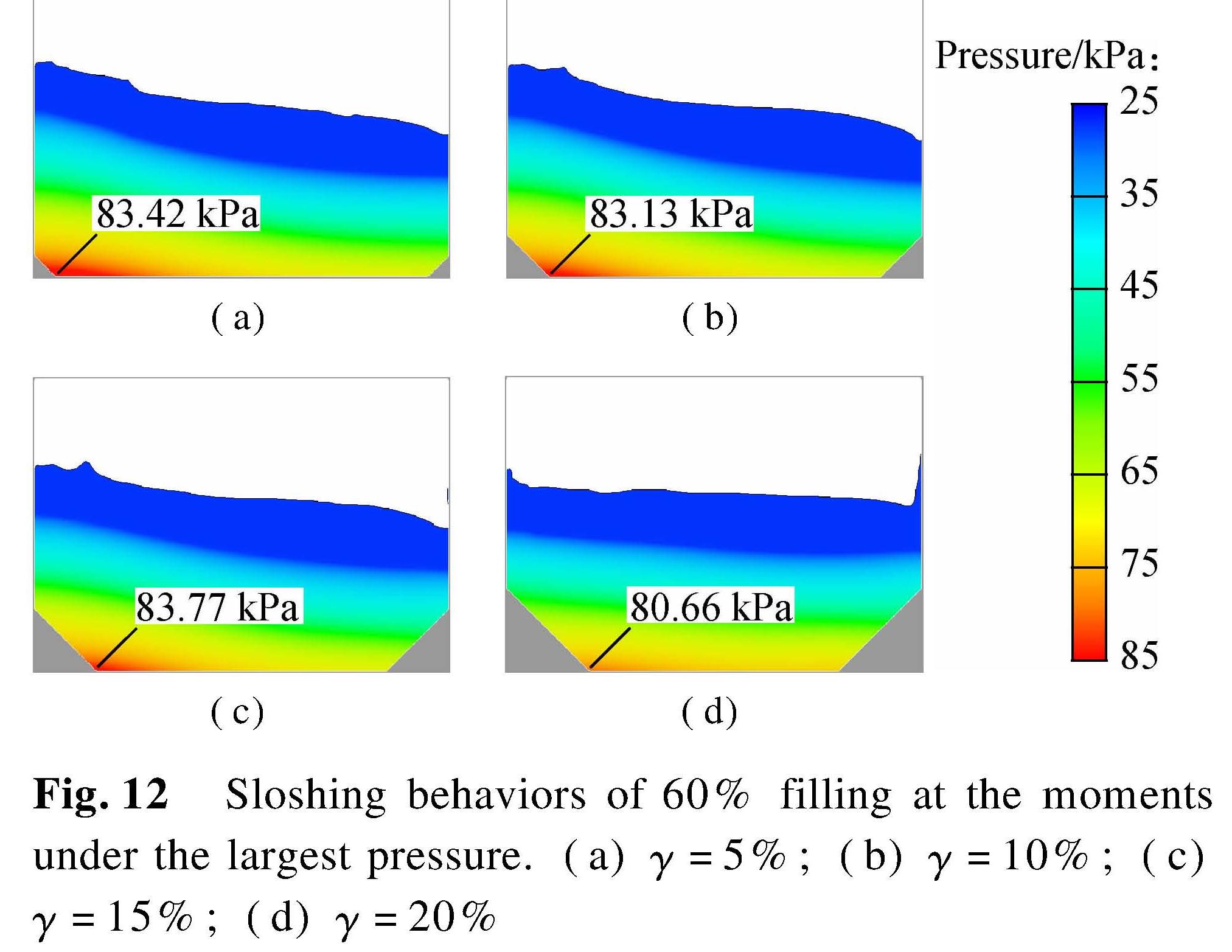
Fig.12 Sloshing behaviors of 60% filling at the moments under the largest pressure.(a)γ=5%;(b)γ=10%;(c)γ=15%;(d)γ=20%

Based on the comparison between the two filling conditions, it can be concluded that the slope size does have some influence on the liquid sloshing behavior and can improve the pressure environment on tank walls. However, this improvement is more obvious at lower filling rates. When the container is filled with more liquid, both pressure improvement and natural frequency will be stable and independent of the change of the slope structure.

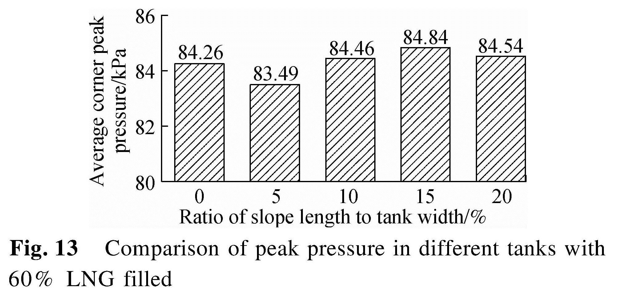
Fig.13 Comparison of peak pressure in different tanks with 60% LNG filled

1)The natural frequency can be determined by the average peak value of hydrodynamic parameters. Therefore, the influence from some extreme moments can be minimized.

2)Three methods are compared to investigate the variation tendency of the natural frequency caused by various sloped bottoms. Due to the accurate prediction in larger slope structures, the average peak method is highly recommended for studying complicated containers.

3)At high filling rates(60%), pressure loading is stable and independent of the change of the slope length radio. However, in a 40% filled tank, the peak pressure on the wall decreases by 5.45 kPa(7.4%)with the increase in the slope size from 5% to 20%, which indicates that 20% slope length ratio is better for reducing the impact from sloshing.